Summary of Bot Ross
Bot Ross is a 2-D contour plotter that draws images with ~1mm resolution using two stepper motors for X/Y movement and a servo for Z-axis pen control. A PIC32 microcontroller manages motor actuation via UART input from a Python script that processes images using Canny edge detection and depth-first search for curve generation. The system faces challenges with mechanical warping and friction-induced step loss, which were mitigated through software adjustments.
Parts used in the Bot Ross:
- PIC32 microcontroller
- Two stepper motors (1.8°/step and 0.9°/step)
- One servo motor
- Texas Instruments SN754410NE quadruple half-H driver IC
- ULN2003BN Darlington transistor array
- Lead screw mechanisms
- Drawer slide
- Alligator clips
- Rack and pinion gear
- Plywood base
- Serial to UART USB adapters
- TFT display
Introduction
Bot Ross is a moderately sized 2-D contour plotter, capable of drawing images with a resolution of roughly 1 mm. The design consists of a pen with degrees of freedom in the x and y directions, actuated using threaded rods controlled by two stepper motors. The pen may be raised or lowered using a small servo motor. The motors, image interpretation, and pen servo are all controlled using a PIC32 microcontroller, while image processing occurs separately using a python script. The idea for this project came from an interest in the applications of a system with two degrees of freedom along a horizontal and vertical rail. A machine capable of reproducing images was a natural application for this kind of structure. The design exhibited its own sort of artistic style based on the linear interpolation between each point in the image, and based on how the images were processed. This is the perfect product for someone who wants to draw pictures, but has limited artistic talent.
High-Level Design
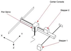
xy-Plane automation robots have become increasingly prevalent in industry as well as in the hobbyist space and served as the main source of inspiration for this project . From laser printers to homemade CNC machines, the market for these robots is always expanding and we thought that a foray into the robotics space would be not only an extremely relevant project but one that would give us a sufficient challenge. Instead of developing a pick-and-place machine as we originally intended, we opted to create a 2D draw bot that was able to take images that would be preprocessed on a computer, uploaded to the PIC, then drawn. This project was hardware focused, and required thought behind construction of not only the motor drivers, but the entire mechanical assembly. Not only was it physically nontrivial, actually drawing the curves provided by the computer or even taking input from the computer would be nontrivial as well. Initially we were faced with the tradeoffs between price, accuracy, and size. When looking into stepper motors, we quickly realized that we could only choose between two of the three previous categories, hence our decision to make the robot large. This increase in size allowed the proportional error of the system to be relatively low as fractions of millimeters would not be recognizable across multiple decimeters. In the end, we opted to use three motors, two steppers and a single servo, all driven by the PIC32. The hierarchy of our project is shown in the diagram below.
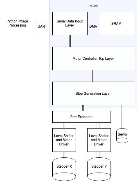
As shown above, we first take an image on a computer and process it using our own python script that uses edge detection and curve generation algorithms to package the image in a format that could be read and processed by the PIC. This would then be transmitted from the computer via a UART connection to the PIC, where it would be stored in the SRAM of the PIC. Once a full transmission was received, the PIC would enter the Motor Controller Top layer where it would run a linear interpolation algorithm to drive the Step Generation Layer, which would actually generate the control signals required for the stepper motors as well as the actuation of the pen servo motor.
Program/Hardware Design
Stepper Motor Control:
As the component responsible for the entire project’s motion, the ability to precisely and simply drive stepper motors was imperative. Stepper motors were favored over DC motors because of the capabilities for accurate open-loop control. Designing a closed-loop feedback system in two translational directions would have been a time-consuming challenge, and one made unnecessary with a good open-loop control scheme. Since each motor could be specified to turn a very specific number of degrees, it is possible to always keep track of the pen’s overall position when applied to this project. This requires the ability to actuate the stepper motors as close to one step at a time as possible, which were 1.8°/step for the motor controlling y-direction motion, and 0.9°/step for the motor controlling x-direction motion.
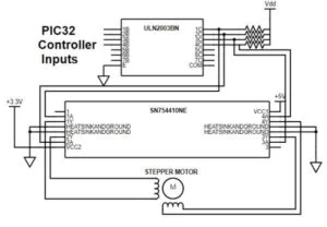
To use our two bipolar, 4-wire stepper motors, it was necessary to include H-bridge circuits to create bidirectional drive currents. To do so, a Texas Instruments SN754410NE quadruple half-H driver integrated circuit was used. This IC is most commonly used as a driver for stepper or DC motors. The half-H driver ran on a 5V logic level, and included a power line which we set to 3.3V to power the motor. Microcontroller inputs are inputted to pins 1A, 2A, 3A, and 4A, with resulting drive currents outputted from pins 1Y, 2Y, 3Y, and 4Y. This allows either stepper motor inductor to be driven with a pair of H-bridge outputs, paired based on corresponding microcontroller inputs. In this case, one inductor was driven using 1Y and 2Y, while the other was driven with 3Y and 4Y. Additionally, each microcontroller input needed to first be level shifted up from 3.3V to 5V, as the driver IC required a 5V logic level. To do so, a ULN2003BN Darlington transistor array was used. This IC was used to build a series of four BJT logical-not gates. By wiring microcontroller inputs to the base and a 5V source through 2kΩ pull-up resistors, the inverse of the microcontroller signal was sent to the half-H driver at 5V rather than 3.3V. Below is a full schematic of the hardware to drive one stepper motor:
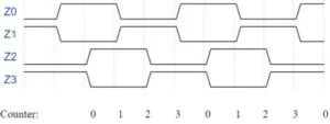
With the motor driver hardware in place, control signals generated from the PIC32 microcontroller could be applied. Two pairs of signals were required to drive a stepper motor, where each pair was simply a square wave and its inverse. Each drive signal was generated using a timer-based interrupt service routine to toggle port expander pins to high or low values. An interrupt timer was used rather than an output compare channels due to the out-of-phase nature of the driver input pairs. In order to step the motor most effectively, each of the motor’s inductors needed overlapping signals sent to each, as shown in the waveform diagram below, where port expander outputs Z0-Z3 were connected to transistor array inputs B1-B4, respectively.
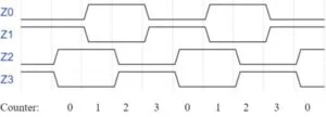
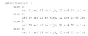
To generate the above pattern, an interrupt service routine ran using interrupts from the PIC32 microcontroller’s timer 3. The ISR ran at 83.33 Hz, a frequency determined by a combination of testing and stepper motor documentation noting that the stepper motors in use typically operate with drive signals at 100 Hz. As shown in the above diagram, a counter variable from 0 to 3 was used to distinguish four states for the drive signals. Its value was initialized to 0 before initiating a motor step. Each time the ISR ran, it would set the appropriate pins to high or low depending on the value of the counter variable. Below is an example of the code structure used in the ISR to generate the above waveform:
Since the ISR is constantly running, control logic is required to determine when to actually step the motors. This is accomplished using a binary valued variable is_step, which signifies whether a step is in progress and/or desired. To initiate stepper motor motion, this value is (externally from the ISR) set to 1. The ISR code to set port expander pins then runs conditionally based on whether this value is true. After I/O pins are set, this value is set back to 0. A program external to the ISR must re-assert the value of is_step in order to continue motion, or leave the value at 0 to stop motion. Another consideration is the direction in which the motor will spin. The above diagram is only capable of producing one direction of rotational motion. By swapping the drive signals Z0 and Z1 with Z2 and Z3 (indicated by the diagram below), respectively, the motor will rotate in the opposite direction.
Motor direction is indicated by another binary-valued variable, where a 1 corresponds to the first set of waveforms, and a 0 corresponds to the second set of waveforms. To generate all of these patterns in software, another instance of the logic structure described above is added to the ISR. The additional code sets I/O pins corresponding to the second waveform diagram rather than the first. Each runs conditionally based on the direction variable. The software as described above is effective in stepping a single motor – however, this project involves two motors. In order to actuate both independently, the code as described above is copied within the same ISR, Variables to control direction and motion are also duplicated to independently control each motor. The copied code uses port expander I/O pins Y0-Y3, along with a second level-shifted H-bridge circuit for the second motor.
Because it takes three ISR hits to generate a cycle for each of the drive signals, it follows that is_step must be re-asserted four times in order to generate one motor step. Furthermore, while testing the motors’ motion, it was determined that it took multiple motor steps to achieve any meaningful actuation. Therefore, it became necessary to implement a user-friendly interface in software for motor control. This was implemented by creating functions, one for each motor, meant to be spawned as new threads when called. Each function takes two arguments, defining both the motor’s direction and how many meaningful steps to take. The structure of a motor step function is described in C-based pseudocode below:
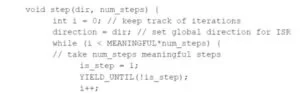
The value MEANINGFUL refers to the number of ISR hits it takes to produce a motor step which we define as one unit in either direction. This allows this function to re-assert the is_step variable the correct number of times to move each motor enough to actuate the system the desired number of steps. With experimentally-determined values of 50 and 27 for the x-direction and y-direction motors respectively, spawning a thread with the step function would actuate Bot Ross’ pen about 1mm using a num_steps argument equal to 1. Again, this function was implemented in two versions, one for each motor, where global variables used by the ISR are set accordingly based on which motor’s step function is being called. These functions implement a programming interface to be used when actually drawing an image, as any specifics pertaining to hardware or drive signals are abstracted. This allows us to draw images by sequentially spawning threads which essentially tell the motor, “move in this direction however many times”.
Physical Construction:
Our robot implemented three motors so that it could actuate on three degrees of freedom. The choice was made to go with stepper motors for the higher precision requirements of the x and y axis. Stepper motors were chosen as they are able to function in open loop systems as each step generates a predictable turn in degrees as opposed to a DC motor which is free running. By coupling the stepper motors to lead screw mechanisms, we could translate the rotational motion of the motors to linear motion along the axis of the screw. One stepper motor was attached to an arm threaded through the first lead screw so the entire second lead screw assembly could be actuated in the ydirection. This arm is suspended on one end by the lead screw and on the other end by a drawer slide. Each lead screw was terminated in our own custom made lead screw holders, which are simply supported with a hole where the screw rests. Once the second lead screw was successfully mounted to the first, we were able to traverse the entire xyplane in a large area, almost 12’ by 12’.
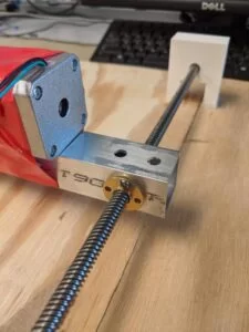
With motion in the xyplane, we needed a way to actuate the pen in the zdirection so that we could lower and raise the pen on command. This was done by fixing two alligator clips to a rack and pinion gear which was actuated by a servo. A servo motor was chosen for this as the degree of precision was not of high concern when considering the use of a felt tipped pen as well as the low tooth count in the gear. Shown below is the final revision of the center console that was used in the finished project.
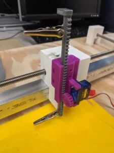
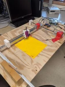
The entirety of the assembly was then taken and glued down to a large piece of plywood which served as the base for our robot. This however was the cause of multiple headaches later on as the board was extremely warped. Below is a picture of the full assembly of our project.
Serial Input:
The connection between the image processing and the PIC32 is handled by a UART connection using the Serial to UART Usb adapters used in Lab 3. These adapters allow for low level access from a computer to the PIC and, when providing the write combination of strings, allow the PIC to receive the images being processed by the python script. For the proper input of the image files, we first made a buffer for the images to be stored on the PIC, which is shown below.
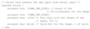
We opted to use unsigned char as the data type to store the coordinates for the image, as the max resolution that we could output was 200×200 pixels as defined by the image processing script. Originally we used unsigned ints, which used four times the memory on the PIC and we would not have been able to store a full image. This reduction of memory allowed us to expand the size of the buffer to 5000 coordinates per image, essentially allowing the PIC to store the full image on the onboard SRAM. This buffer would be filled via the DMA channels on the PIC utilizing the serial library in the provided protothreads implementation. Using PT_GetMachineBuffer, we created the state machine shown below to receive the incoming information from the Desktop.
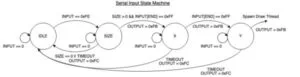
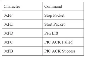
First, the computer sends an initial package that contains a start character, then sends the size of the incoming image in chars. To ensure proper communication between the host (Computer) and the receiver (PIC), we developed a rudimentary communications protocol with ACK bytes to ensure that each packet was being successfully transmitted. Below is a tabulation of the values that we assigned commands, knowing that we had (28-1) -200 characters available for use. As well as the table, there is an example packet from the host to PIC.
Once the size packet was successfully received, the PIC then looks for the x coordinate packet followed by the y coordinate packet, which are promptly stored into the buffer variable of type img. Finally, once the image is successfully received, the valid bit is set to high and the serial input thread spawns the draw thread which begins to draw the received image.
Image Processing
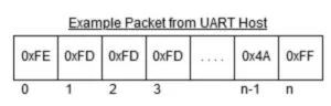
Bot Ross is an edge contour plotter, meaning that it is able to plot extracted edges from any kind of image, generating almost an outline of the original. To do this, the system makes use of Canny edge detection done through the OpenCV Python library. The Canny algorithm passes an image through several filters and transformations with an ultimate process of hysteresis thresholding, which results in prominence in color of pixels at edges. When the edge detection library was first tested on the sample images, it seemed to work well, but not in the context of the Bot Ross system. It was apparent that the edges of the image were found, but the edges were all very short and scattered, and it was evident that drawing the pixels in the image would take an extraordinary amount of time. An important part of the edge detection is that the output from the Python script must be an image with a small enough amount of continuous curves to be drawn because the stepper motors do not move quickly. So, it was necessary to process the image to resolve this issue by changing its resolution and modifying its pixels. The image was first blurred, as this helps obtain proper output from the Canny algorithm. After processing with the Canny() function from the OpenCV formula, steps were taken to “connect” the scattered edges and reduce the number of continuous curves to be drawn. First, the resolution of the image was dropped by a certain factor, reducing the actual size of the pixel gaps in the image. Then, for every white pixel present in the image, its neighboring 8 pixels were also colored white if they already were not. The image resolution was then increased using linear interpolation, and this effectively reduced a substantial amount of the empty space that resulted from the original processing. A threshold value of 150 was used for the pixel color value, meaning that every pixel with a value greater than or equal to 150 was added to the coordinate array for plotting.

To generate a list of coordinates to be plotted, a depth first search implementation was used to generate a sequential list of coordinates that also included encoded instructions for lifting the pen off the paper and putting it back down to draw. A loop was used to check every pixel, and if it had a value greater than 150, depth first search would be executed with that pixel as the start of another curve. The implementation worked recursively, so for every call to the depth first search function, if the pixel value was 150 and it had not been visited, it would be added to an array of tuples of visited coordinates. After this, the neighbors of the pixel would be checked, and if it satisfied the conditions, its coordinates would be added into the array and depth first search would be run from there. Within the condition for checking each of the eight neighbors, there is a call to the depth first search function for the corresponding neighbor. After a pixel with no neighbors to be added to the coordinate array has been reached, the recursive function calls will end and the stopping coordinate of (253, -53) will be added. Technically, the stopping coordinate is (253, 253), but since the y-coordinates are flipped by being subtracted from 200 to draw the image upright, the y-coordinate of the appended stopping coordinate is -53. This stopping coordinate is parsed on the PIC as an instruction to lift the pen up and move to the next starting coordinate before putting the pen back down. The visited coordinates array was then split into x- and y-coordinate arrays to be sent to the PIC through serial.
Drawing the Image
To draw the provided coordinates, a simple error function is used to step the motors in appropriate directions to reach the target coordinate. For example, consider that the pen is moving from a position of (x1, y1) to (x2, y2). Every time the thread is run, the errors of |x1-x2| and |y1-y2| are checked, and if either are not zero, the motors will step in a manner that decreases both errors. When drawn, this generates a drawn segment resembling a staircase pattern followed by a straight line. However, since coordinates adjacent in the array often differed in x-coordinates by only 1 unit, this error function did not significantly distort the outline of the image. To stop drawing between curves, the thread checks if the next coordinate is equal to the value defined as the instruction to lift the pen. If this is true, the pen will be lifted and moved to the start of the next curve before being put back down on the paper. Since the serial communication was not fully functional at the time of the demo, a header file was used to store the array of image coordinates. The values for the x- and y-coordinates were copied and pasted into the header file by saving the array output from an execution of the Python script.
After a test run on a processed image, a discrepancy was discovered in how the image was actually being drawn. Parts of the image seemed correct, while others were shifted and out of place, and this was quickly determined to be a hardware issue by comparing the actual coordinate location of the pen to the location it should have been in, displayed on the TFT. Due to the low torque of the stepper motors, the kinetic frictional force of the pen being pressed down on the paper caused some steps to be “lost” when the pen was moving. The implementation depth first search prioritized moving up and to the left, so when the pen was put back down and moved more to the right, the error from lost steps grew and shifted parts of the image to the left.
The Adjustment:
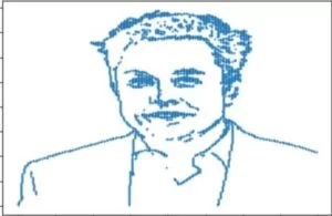
To fix the position error generated by the friction of the pen, we performed an experiment to determine to what degree the pen deflected the step length of the motor. First we drove the pen 150 steps, determining that the pen moved 0.84mm/step. We then dropped the pen and repeated the same track, and measured the difference between the two. The results of the test are shown below.
Initially we thought that the distance between the two lines wouldn’t create the drastic effects that we were noticing. However, after running the numbers this was not the case.

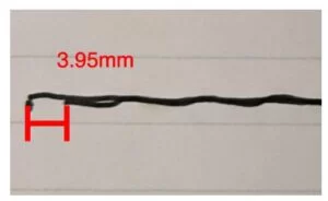
Once we determined that after every 30 steps with then pen down, we generate an error of one step, we realized that this error would completely throw off the image. For an image of over 2000 points, like the Elon picture that we used to test our robot, the xaxis could drift over four centimeters. To fix the problem, we added the following lines of code to step the pen one more time to the right if we have already stepped 30 times with the pen down to the right.
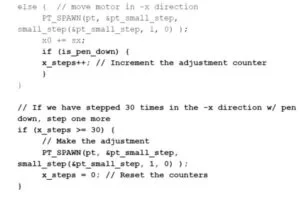
This adjustment worked to correct the accumulated error due to the way that our image processor generates the curve. When the pen is up, the algorithm dictated that the system move to the left most often, due to the backtracking nature of a depth-first search. Our adjustment technique corrected the cumulative error that this feature caused. Shown below are two pictures of Elon, one without the adjustment and one with the adjustment.
Results
By using a linear interpolation between edge-detected image coordinates, along with ~1mm precision provided by our stepper motor programming interface, Bot Ross was able to draw sketches of images with admirable accuracy. Below is the finished product of an image we used while testing our design, alongside the original image:
The image took about 15 minutes to draw. Draw times will vary based on the image, and more importantly, how the image processing/curve generation algorithms represent the image to the PIC32 microcontroller. Aside from the difficulty to capture details when using edge detection to draw images, mechanical inconsistency was the main source of inaccuracy. Fortunately, no interference came from other projects/surroundings.
The serial terminal, unfortunately, was not functional at the time of demonstration due to an error with the counting of the size of the incoming image. This would cause the serial communication link between the PIC and the computer to exit prematurely so the image could not be loaded onto the PIC. This is most likely due to the semantics between the library being used for the serial communication on the desktop in python, the Serial to Uart connector, and the PIC. To debug we reinstalled the tft in an attempt to get a better idea of what was going on within the PIC, but we still could not quite get the serial communications working. Moving forward, this would be the first thing that would be improved or fixed within the project as it is already close to full functionality.
For demonstration, images were loaded from the python script to the PIC32 microcontroller by declaring the image’s x and y arrays in a C header file, using the const keyword to store it in flash memory. This design is suboptimal in terms of usability, since it requires reprogramming every time a new image is drawn. This was the purpose of using serial communication between a laptop running our python code and the PIC32 microcontroller. This would have provided the desired user-friendly functionality, explained in the following steps:
- Save image file on a computer
- Plug microcontroller into computer, determine which COM port it is recognized as
- Run python script, which prompts the user to type in the image name and appropriate COM port
- Enjoy watching Bot Ross draw!
Conclusion
The function of Bot Ross almost reached our target goal set at the beginning of the project. The system drew images exactly the way we intended for with the exception of serial communication between the computer and the PIC. We ran into several errors and malfunctions in the system along the way, but we were ultimately able to resolve these issues by the time of the demo. We were satisfied with the resolution with which the system was able to draw images, because we originally believed that the rasterized form of the image would not resemble the original image well. However, considering the scale of the drawn image to the displacement of the pen from one step in either motor, a rasterized form still works well when drawing an image. A change we would make to the current system is in aspects of its mechanical design. The wooden platform used to mount the motors and drawer slide was slightly warped, and this affected the pen down state because the force of the board against the pen was not constant. The warping of the platform also affected the stability of the drawer slide, because the slide often fell off as the small motor arm moved back and forth in the y direction. 2D plotters have been around for quite a while and now are made to be extremely precise, so Bot Ross did not match up to plotter systems that exist now and can be purchased. Yet, Bot Ross drew with significant accuracy, and it was interesting to see how different images translated to their drawn version on paper.
Some of the code for this project was obtained from external sources. The code for Canny edge detection is from a function in OpenCV, an open source computer vision library. To implement different threads, the Protothreads library was used. Much of the code to use the Protothreads library, port expander, and PIC was provided by Dr. Bruce Land through the course material available to us. This website was designed with help using an open source template from Start Boostrap.
For safety, Bot Ross should be used under supervision from a safe distance to ensure safety with mechanical parts, which could pinch the skin while moving.
The unique use of depth-first search for curve generation is proprietary, and treated as our intellectual property. All other code may be used generally and treated as open source, considering it has likely been implemented for similar applications.
Source: Bot Ross
- How does Bot Ross draw images?
The system uses a Python script to process images via Canny edge detection and depth-first search, then sends coordinates to a PIC32 microcontroller which drives stepper motors. - What components control the pen movement?
Two stepper motors control the X and Y axes, while a servo motor controls the Z-axis to raise or lower the pen. - Why were stepper motors chosen over DC motors?
Stepper motors allow for accurate open-loop control where each step generates a predictable turn in degrees. - How are motor signals generated by the microcontroller?
An interrupt service routine running at 83.33 Hz toggles port expander pins to create square waves and their inverses for bidirectional drive currents. - What issue caused image shifting during drawing?
Low torque stepper motors lost steps due to kinetic frictional force when the pen pressed down on the paper. - How was the cumulative error fixed?
The code was adjusted to step the pen one additional time to the right after every 30 steps taken with the pen down to the right. - What communication protocol is used between the computer and robot?
A UART connection with a custom protocol using ACK bytes ensures successful packet transmission of image data. - What algorithm is used to generate continuous curves?
A depth first search implementation generates a sequential list of coordinates including instructions to lift and lower the pen. - Can the robot draw images directly from a laptop without reprogramming?
Theoretically yes via serial communication, but the project demo required copying coordinate arrays into a C header file because the serial link was not fully functional. - What mechanical problem affected the accuracy of the build?
The warped plywood platform used as a base caused inconsistent pen pressure and instability in the drawer slide.