Summary of Automatic Signal Transformer and Custom Filter Designer
This project implements a touchscreen-driven custom FIR filter designer on a PIC32 that lets users draw a desired frequency response, interprets pass/stop bands, computes FIR coefficients via Parks-McClellan or frequency-sampling (FFT-based) methods, and performs real-time convolution of ADC-sampled input to a DAC output for live demonstration. The system includes touchscreen input, ADC sampling, SPI DAC output, and a Protothreads state machine managing drawing, processing, filter design, and real-time output.
Parts used in the Automatic Signal Transformer and Custom Filter Designer:
- PIC32 microcontroller
- 10-bit ADC (internal to PIC32)
- MCP4822 12-bit DAC
- Resistive PiTFT 320x240 touchscreen (Adafruit)
- SPI interface
- External pushbutton (interrupt on RB7)
- Timers (Timer2 and Timer3 on PIC32)
- Signal generator (input source)
- Oscilloscope (output measurement)
- Protothreads cooperative scheduler (software)
This laboratory aims to implement a custom filter designer on the PIC32 microcontroller for the purpose of real time signal transformation. The project gets its premise out of the frequent requirement for arbitrary digital signal filters in a laboratory setting. For a video of our lab demo please see Project Demo
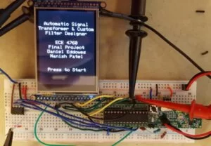
A user is given the ability to draw a transfer function on a touchscreen interfaced with the PIC, a custom interpolation and interpretation algorithm is used to understand the essential pass and stop bands of the users transfer function. These bands are used as the argument to either a Parks- McClellan or Fourier Transform algorithm which creates the discrete time impulse response coefficients corresponding to the drawn frequency response. With discrete time finite impulse response (FIR) filter coefficients a real time convolution is taken with an analog to digital converter sampled input signal and then output to a 12-bit digital to analog converter. In this way, a user can design their filter and see it implemented in real time. Pictured blow is a figure of the entire system, with input from a signal generator and output to an oscilloscope off-screen.
High Level Design
Rationale
The source for this project idea was Bruce Land, who thought that it would be a good idea to make a project that allowed users to specify arbitrary filter transfer functions that could be used for digital signal processing. The creators of this project also believed that this would be a fun and challenging project, and decided to undertake it.
Logic Structure
A high level block diagram that describes the logical structure of the project is shown below.
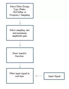
Essentially, the logical flow of the program is as follows. First, the user decides whether or not they would like to use the Parks-McClellan algorithm or the Frequency Sampling Algorithm to design their FIR filter. After that, they can set the sampling rate and maximum amplitude of the transfer function plot that will be displayed on the touch screen. Next, they draw the desired transfer function on the touch screen. At this point, the chosen algorithm will begin to run in order to generate the filter coefficients corresponding to the drawn frequency response. Once the coefficients have been generated, the input signal will be convolved in real time to produce the output.
Hardware & Software Tradeoffs
The main tradeoff in this project between hardware and software is the debate between digital and analog filtering. Theoretically, all signals can be filtered in hardware. However, this requires the user to know a priori exactly what type of frequencies need to be filtered. The choice to filter in software, which is more computationally intensive, allows for greater flexibility for the user to determine exactly how they want to filter their input. Thus, in terms of hardware and software tradeoffs, computational speed and execution time is sacrificed for greater modularity.
Hardware Design
Overview
As will all the labs in this course, the PIC32 acts as the logical backbone for the entire system. A signal is input to the PIC through a 10-bit analog to digital converter (ADC) internal to the PIC32. The filtered signal is then output as a 12-bit number to the MCP4822 digital to analog converter (DAC) over a serial peripheral interface (SPI). The DAC outputs an analog signal representation the filtered input. During the creation of this project a sinusoidal input from a signal generator is used as the input to the system, and an oscilloscope is used to measure the DAC output. A schematic of the whole system is in the Appendix following the report.
ADC & DAC
The system used three ADC channels. Namely, AN5 (port pin RB3) and AN11 (port pin RB13) to read the Y and X axis of the touchscreen respectively, as well as AN0 (port pin RA0) for the signal input. AN0 is not set at the ADC channel until it is time for convolution to take place inside the state machine. The ADC input and DAC output occur at the Nyquist rate of whatever input frequency the user selects from a list. They are contained within timer 2 and timer 3 match interrupts respectively. These timers are turned on at the same place the ADC channel is set to AN0. In this way interrupts only take cycles time away from the executing program when it is absolutely necessary.
Touchscreen
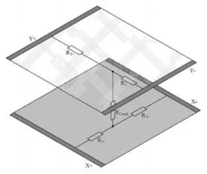
The user drawn transfer function occurs on a resistive touchscreen, the PiTFT from adafruit. The touchscreen used in this lab is a standard 320×240 resolution resistive touchscreen. A simple SPI interface is used to write data to the screen. Two resistive sheets are located on top of a TFT display. When a touch is applied to the screen, the sheets touch and a voltage divider is created which is measurable through the PIC32s ADC. To determine a touch coordinate, power is applied to one sheet and voltage is read off the other, the location of the touch will result in larger or smaller division of the voltage divider and result in varying output voltages. The process is then flipped, the other sheet is powered and the ADC is used to measure the divided voltage off the other. An image of a generic resistive touchscreen is shown below.
A significant delay on the order of 10 ms is used in between switching which sheet is powered in order to allow outputs to stabilize. This effectively reduces the touch points per time resolution to under 50 times per second. This however is of little concern because at the end of the day, a human will never be touching the screen that fast.
The actual coordinate of the touch is represented as two 10-bit numbers, following directly from their ADC measurements in either direction. Some scaling is necessary to get this back to a pixel location, however to speed computation values relating touch points to screen positions are often hard coded as their ADC instead of pixel value. Due to manufacturing defects and the nature of the two resistive sheet geometry of the touchscreen, high and low ends of the 10-bit spectrum are impossible to obtain when determining touch location. For this reason an additional check and consideration has to be made to make sure a touch point is in the physically viable range of the screen.
External Interrupt
An external button is used to initiate an external rising edge interrupt on pin 16 (RB7) of the PIC32. This interrupt is used to stop convolution and return program execution to its start state. As will be examined more, convolving the ADC input with an FIR filter is a real time process and is therefore best interfaced with through an interrupt service routine. An external button is used to trigger the interrupt because of its ease of implementation is software and speed with respect to the touchscreen display. The button is tied to ground via a capacitor in order to ensure that the input to the PIC32 does not float and to reject noise from programming or the sinusoidal input, located close in proximity to the button on the white board.
Software Design
Overview
This project is primarily a software intensive digital signal processing exercise. It is divided into three major design components; the touchscreen and drawing the filter transfer function; Parks McClellan and Fourier Transform algorithms and determining FIR filter coefficients; and the real time convolution with signal output. Each component is addressed individually but first it is worth investigating the software structure. The executing program is scheduled according to the Protothreads cooperative scheduler. This project uses two such threads, one to handle touchscreen reading and data parsing, and another to facilitate a state machine.
State Machine
The state machine operates linearly; first collecting user data, like what sort of transform and particular parameters the user would like to use, and then moves to drawing and processing the transfer function, and final computing filter coefficients and outputting the signal. State machine is shown below.
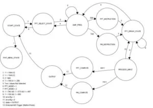
As evident in the above image, most of the transitions from state to state occur according to specific areas of the screen being touched. Although the error and transform mode flags also play a role in traversing the machine. Here is a walkthrough of each state and the basic progression through the program.
STATE_START
Here the user selects their desired transform type, Fast Fourier Transform (FFT) or Fast Wavelet Transform (FWT). It was a reach for the project to encompass a wavelet transformation, and it remains unimplemented. Touching the half of the screen corresponding to the user’s desired transform will advance the state. Pictured below is the TFT display for this selection screen.
FFT_SELECT_STATE
Much like the previous state this allows the user to select between two different Fourier transforms, a standard FFT, or a more complex but also optimized Parks McClellan implementation. Much more on both types of transforms later. Again, simply touching the half of the screen corresponding to the desired algorithm will advance the state. Here however, pressing a back button located in the top left corner of the screen will return the user to STATE_START. Below is an image of the TFT display at this state.
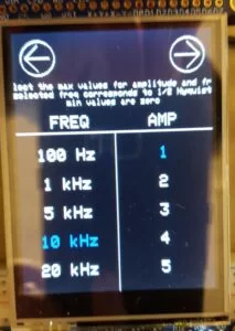
AMP_FREQ
This state has the user select two values, the maximum frequency and amplitude to be used in the transformation. The frequency selection will scale the ADC read period to twice the selection, the Nyquist rate for the particular input. In practice frequencies can be processed up to 40 kHz. The amplitude selection will set the maximum amplitude on the transfer function that the user eventually draws. The user has to be mindful of the amplitude of their input because although the program gives them the ability to amplify up to 5x the input, clipping will occur after a 3.3V output.
By touching the number according to the desired frequency and amplitude selection the parameter is stored in memory. The text on screen will also turn blue, indicating a selection. If the user wishes to change their selection they simply need to press another number. The original selection turns white and the new selection turns blue. This is meant to be as intuitive as possible for the user.
By pressing the back button in the top left of the screen the user can return to the FFT_SELECT_STATE at any time. The top right of the screen houses a forward button that advances the user to the next state. If less than two values, one frequency and on amplitude value, are selected, the state throws an error indicating such and loops back onto itself.
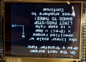
PM_INSTRUCTION & FFT_INSTRUCTION
Upon pressing the forward button from the AMP_FREQ state, the user is presented with a series of instructions on how to draw the transfer function on the next screen. Instructions are unique depending on which state is pressed. Pressing the screen again continues the user to the next state. The instructions specific to the Parks McClellan transform are shown below.
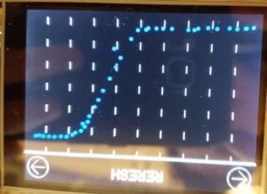
FFT_DRAW_STATE
This state starts be rotating the screen by 90 degrees counter clockwise, giving the user more screen real estate along the x-axis (frequency). They are then tasked to draw a transfer function. The x-axis is scaled from zero to pi along a 320 pixel range, as any transfer function is, and is drawn with dashed lines at intervals of one tenth pi. The y-axis is scaled to take up exactly 200 pixels on the screen according to the max amplitude selection, and a dashed line is draw from every integer of that selection.
The user can then simply draw whatever plot they would like across the screen. Every coordinate input that is detected on the touchscreen is replayed by drawing a circle. There will inevitably be gaps when drawing because of the computation involved in plotting to the screen and the naturally required delay in the screen. This is fixed a little later down the line. An example of a transfer function drawing is shown below.
A Refresh button in the top middle of the screen resets the state, this resets the state and allows the user to draw their function again. Again a back button will return the user to the previous state, in this case AMP_FREQ, and a forward button will advance the user to an animated state, PROCESS_INPUT, which cleans up their transfer function and gets it ready for filtering.
PROCESS_INPUT
This state fixes the drawn transfer function by eliminating errors, filling gaps, and checking for potential errors in the plot. Please see the Transfer Function Interpretation section below for a complete walkthrough. If an error is not detected the state machine will continue to filter computation automatically. If an error is detected, the state machine will return to FFT_DRAW_STATE where the user can fix what was incorrect.
PM_COMPUTE & FFT_COMPUTE
These states generate the FIR filter coefficients. A filter mode flag set in code determines which algorithm to use. Please see the Filter Design section and its subsections below for more information.
Upon displaying ever coefficient, the state machine automatically advances to the OUPUT state. First is enables timers and interrupts to handle ADC input and DAC output, without these nothing would pass through the system. It is here that DAC and ADC interrupts are enabled and the ADC channel is updated from that of the touchscreen to the input signal channel. At the end of this state the system has all of the FIR coefficients necessary for real time convolution. After execution it defaults to advance to the OUTPUT state.
OUTPUT
This is the final state in the state machine, it is here that the real time convolution between the input signal and the FIR coefficients occurs. No matter the origin of those coefficients, be it Fourier or Parks McClellan, the state operates the same. It first fills up a buffer with input signals of length equal to the filter. Pairwise multiplication and summation occurs between the input and FIR values in real time. By real time it means that the time it takes to compute the convolution takes less time than the Nyquist rate period, and can therefore simulate real time.
The minimum value of the convolution is always maintained and added to the output DAC value if it ever dips below zero. This aims to act as the DC offset of the input signal. Instead of sampling the input for an arbitrary known amount of time and taking a time average to find the offset, this method is much more compact and dynamic.
FWT_MENU_STATE
Mostly a dummy state, just displayed text and allows the user to return to the transformation selection state by pressing a back button.
Transfer Function Interpretation
A user draws their desired transfer function by a series of points along the curve of their desired transfer function. Any time a pixel value is read as an input to the screen it is stored in a 320 element array, which acts as an injective mapping between x-axis pixels and y-axis transfer function values. An element of this array can only be drawn to if it has not been previously, thus this ensures that whatever is draw is a function. Granted this function may be an awful looking 320 element piecewise function. Another dilemma arises when swiping across the screen. If there is an acceleration in the xy plane, as is the case when drawing at a constant velocity then changing directions, the touch screen may misinterpret a data point and accept a fault point as valid. An example of this is shown below where an extraneous value is plotted right when the user leaves the transfer functions pass band and enters a transition region.
In order to correct these errors, fill in gaps, and understanding what is drawn by the user we must assume errors are not purposeful and that gaps contain no additional information. A five element medium average filter is used to remove error points by setting them to the value of their neighbors. Every non zero element in the 320 element array is set to the median of the surrounding two values. This does a fantastic job to smooth out touchscreen outliers. The next step used is a linear interpolation between each nonzero point to the next nonzero point. This fills in the gaps in the bode plot and gives the user a more complete picture of their transfer function. Floating point math is used to calculate slope to ensure than even for slopes within unity magnitude around zero will be mapped and plotted correctly.
A four element moving average is then used to smooth out jagged values and artifacts from interpolation that are undesirable. The slight frequency delay caused by the moving average is negligible compared to the 320 element domain of the screen and so is not a huge concern. After each of these steps the transfer function is redrawn and a blocking delay is used to give the user time to see the changes. In standard Fourier Transform mode this is where the story ends but for Parks McClellan few additional steps are needed.
For Parks McClellan all of the bands in the transfer function are determined explicitly. This is done through an iterative process similar to the one described above with the aid of a discrete derivative. After median filtering, linear interpolation, and moving average filtering, a discrete derivative is used to find the change in amplitude on the transfer function per 4 pixel x-value change. If this derivative term is within a threshold, which through repeated experimentation is 3 pixels, then it is kept in the transfer function, else it is thrown out. This relies on the fact that each band wills be relatively linear (if not zero in slope) but distinct from the other bands by a significant amplitude margin.
This pass will usually determine the bands fairly well, but due to the aforementioned touchscreen artifacts there are occasionally measured bands in the transition regions. To fix this problem the entire process is repeated one more time. On top of this, because of Parks McClellan stipulations (more on these later), transition regions must be greater than one tenth of pi in length, and not pass/stop band can begin after .8pi. If an error is caught the user simply touches the screen to reset the function and are instructed to redraw. These checks are not only in place to ensure that the Parks McClellan math will be performed successfully, but the often catch faulty registration of pass and stop bands.
Once the process has been carried out twice and errors have been checked for, the algorithm is complete. In practice it is fairly robust and stable against absurd input and abnormal touchscreen errors.
Stepping through the entire 320 element array one more time, the pass/stop band endpoints are determined via a discrete derivative and are then averaged to determine the amplitude value within each band domain. All of the bands are then scaled according the amplitude specified by the user. Below is an image of the transfer function after the entire algorithm has been run. Blue dots indicate the function, red dots indicate the return from the discrete derivate plotted along the function, and the green dots indicate band regions. To see all of this, below are two images of the same function. The first one is the function unfiltered, the second is of the filtered function, which is ready for filter computation.
With the transfer function known the next set is to develop finite impulse response filter coefficients.
Parks-McClellan Filter Design Algorithm
The Parks-McClellan FIR filter design algorithm is an industry standard algorithm for creating the optimal filter given a desired magnitude for the frequency response. It creates filters that are optimal in the L-infinity sense – that is, it minimizes the maximal error present within the pass and stop bands regions of the filter. This type of filter is called equiripple, since it will exhibit a rippling phenomenon in the bands, where the error of each ripple has constant magnitude and alternates in sign with each ripple (Ref 1). This project implements a limited form of the Parks-McClellan algorithm, which works for optimal design of low and high pass filters. An attempt was made to implement the most general form of Parks-McClellan, which works for completely arbitrary frequency responses, but due to the additional complexity of the algorithm this was not possible to complete within the given time frame. The details of the algorithm are mathematically intense and a completely rigorous description will not be provided in the report. Instead, a more general overview of the major steps will be given.
The first step of the algorithm is to take as an input to the function the desired magnitude of the frequency response that the user has drawn. This limited form of the Parks-McClellan algorithm assumes that there are only two “bands” in the frequency response – that is, two flat regions that indicate wither a pass or stop region. In this way, low and high pass filters with arbitrary cutoff frequencies can be specified. Thus, the function requires an input that indicates the start and end frequencies of each band, and the magnitude of the frequency response at each of these frequencies. This input format is similar to the Mathworks firpm function (Ref 2). Additionally, the desired filter length is required as an input. This implementation assumes a default filter length of 35, which, from thorough testing, seems to be long enough to generate low and high pass filters with a transition band that is at least .1*Pi wide. The steeper the transition region the longer the filter must be to achieve the steeper cutoff.
Once the bands have been specified in the way described, the algorithm can proceed. The first step is to initially assign the set of “extremal frequencies,” or frequencies at which the generated frequency response is supposed to have a maximal error (the peaks and valleys of the ripples). To initially assign this set, it is assumed that the frequencies are evenly distributed within the pass and stop band. The number of extremal frequencies is given by the following equation, where M is the overall filter length:
Thus, in the case where M is 35, the number of extremal frequencies is 19. After evenly distributing these 19 frequencies within the pass and stop band, the next step is to compute the value of delta, which is one of the solutions to a system of polynomial equations that has undergone a cosine transformation. Essentially, the linear system states that the frequency response that the user has specified can be approximated as a polynomial with degree n and a fixed error delta at each of the extremal frequencies. Thus, the goal of solving this system is to determine n+2 unknowns, which are the n+1 polynomial coefficients and the value of delta. To do this, n+2 data points are needed – namely, the extremal frequencies! Thus, this linear system can be easily solved by plugging in the extremal frequencies into the general form of the cosine transformed polynomial (again, refer to the previously mentioned document for a mathematically rigorous treatment of this subject). The full solution to the system will provide the filter coefficients as well as delta, but computing all of these is unnecessary for each iteration of the algorithm; only the value of delta is needed at each iteration. A simple, closed form solution to delta exists that allows one to solve for this value specifically without solving the entire system (Ref 3):
(This implementation assumes a constant weighting function, otherwise the above equation for delta would be slightly different.) The function Ad is the desired value of the magnitude of the frequency response at the specified extremal frequency. w represents the set of extremal frequencies. This equation is far more computationally efficient that solving the system at each iteration of the algorithm.
Although computing the value of delta will tell one what the error at each of the extremal frequencies is, there is no guarantee that after just a single iteration that this error is optimal in the minimax sense. Thus, the next step is to compute the full error function over the entire range of discrete frequencies, from 0 to Pi. This could technically be accomplished by solving the full linear system and then using the resulting polynomial to evaluate the generate frequency response at every point, and subtracting it from the desired user input, but again, this would be computationally inefficient. Instead, lagrange interpolation (Ref 4) using the n+2 extremal frequencies, and the amplitude of the frequency response at each of these points (which is just the desired amplitude plus or minus delta) is used to compute the error function over a set of 16*n data points. The error function is simply defined as the difference between the discretely computed values of the frequency response as generated by lagrange interpolation and the desired magnitude of the frequency response. (According to the Jones paper (Ref 5), interpolation should only be performed using n+1 of the extremal frequencies, but this yielded bizarre results, so all n+2 frequencies were used.)
Once the error function is computed, the next step is to determine the local maxima and minima of the error function, keeping in mind that all of these extrema must lie inside the bands, and not in the transition regions. These new extrema will become the new set of extremal frequencies. If the location of the extremal frequencies doesn’t change, then the process is stopped. If the set of extremal frequencies does change, then the process is repeated over again with the new set (Ref 6). In this implementation, the number of iterations is limited to 10.
Once the algorithm has converged, the final step is to actually solve the aforementioned linear system. While this is computationally inefficient, it only needs to be performed a single time due to the existence of a closed form solution for delta (Ref 7). To solve this system, an efficient LU decomposition implementation created by Philip Wallstedt (Ref 8) is used. (Permission was obtained via email.) Solving this system, as mentioned previously, will give the desired filter coefficients. However, notice that solving this system only yields n+1 values, when the desired filter length is M (2*n+1 values). In order to generate a length M filter, the last n values returned by solving the system (excluding delta) are reversed, and appended to the front of the original list of n+1 coefficients. All of the values are then divided by 2, except for the centermost value in the list (Ref 9). This final action must be performed in order to make the filter coefficients symmetric, which results in a Type 1, linear phase, FIR filter (Ref 10).
Frequency Sampling FIR Filter Design
In addition to the limited Parks-McClellan algorithm, a frequency sampling method for FIR filter design was also implemented. The basic idea behind frequency sampling filter design is this: given a desired magnitude for a frequency response, sample the frequency response at evenly spaced intervals, use a linear phase assumption, and then perform an inverse FFT to obtain the filter coefficients. This idea to use frequency sampling was originally inspired by a lecture from Professor Delchamps at Cornell University (Ref 11). Implementation details and MATLAB code were found on DSP Stack Exchange (by user Matt L), which was then converted into C code for the Pic32 (Ref 12). In this implementation, a length 64 filter is generated. The Microchip library was used to implement the inverse FFT (Ref 13). Sample code on how to perform the FFT using this library was obtained with permission from Tahmid Mahbub (Ref 14). Confusingly, it appears that the inverse FFT in the Microchip library is accomplished by using the FFT function (Ref 15). Using the FFT function in place of the inverse FFT seemed to work during testing, so this anomaly within the library was not questioned. In general, this method is more flexible than the limited Parks-McClellan algorithm that was implemented, but does not produce necessarily optimal filters.
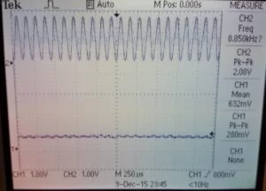
Overall, the code was quite successful. The following tests show the results when an input signal of a given frequency is read into the Pic32 by an ADC, convolved with the filter coefficients generated by one of the two methods specified above, and the result output to an oscilloscope. In all tests, the input signal is sampled at 20 kHz, and the range of allowed amplitudes for the transfer function is from 0 to 1.
Test 1: Parks-McClellan Low Pass Filter
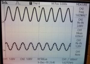
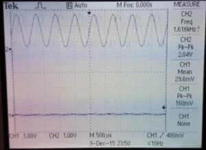
Test 2: Parks McClellan High Pass

Source: Automatic Signal Transformer and Custom Filter Designer
- How does the user specify a filter transfer function?
The user draws the desired transfer function on the 320x240 resistive touchscreen which records x-y coordinates mapped to a 320-element array. - Can the system compute filter coefficients automatically?
Yes; after drawing the transfer function the system processes it and computes FIR coefficients using either Parks-McClellan or a frequency sampling (FFT-based) algorithm. - How is a touch coordinate measured?
The PIC32 powers one resistive touchscreen sheet and reads the divided voltage on the other via ADC, then flips sheets to read the other coordinate using the ADC. - Does the system perform real-time filtering?
Yes; once coefficients are generated the PIC32 performs real-time convolution of ADC-sampled input and outputs to the MCP4822 DAC using timer interrupts so computation finishes within the Nyquist period. - What algorithms are available to generate FIR coefficients?
Parks-McClellan (limited to low/high pass) and a frequency sampling method using inverse FFT are implemented. - How are touchscreen drawing errors handled?
The drawn 320-element array undergoes a median filter, linear interpolation, moving average smoothing, and discrete derivative passes to remove outliers, fill gaps, and identify bands. - Can the Parks-McClellan implementation handle arbitrary responses?
No; this implementation is limited to two-band low-pass or high-pass designs with a default filter length (35) and transition width constraints. - How is ADC channel switching managed for touchscreen and signal input?
The ADC channel is set to touchscreen channels during drawing and switched to AN0 for signal input when convolution begins; timers and interrupts are enabled at that time. - What prevents DAC output clipping?
The user sets amplitude limits and the program warns that clipping occurs past a 3.3V output; amplitude selection scales the transfer function accordingly. - How does the system return to the start state during output?
An external button tied to RB7 triggers a rising edge interrupt that stops convolution and returns execution to the start state.