How to Build a Self Navigating Robot

This is a detailed tutorial on how to realize a robot starting from scratch, and giving it the ability to navigate autonomously in an unknown environment.

All the typical arguments involved with robotics will be covered: mechanics , electronics and programming .

The whole robot is designed to be made by anyone at home without professional (i.e. expensive) tools and equipment.

The brain board (dsNav ) is based on a Microchip dsPIC33 DSC with  encoder and motor controller capabilities. The position is computed by odometry (encoder) without any external reference (dead reckoning).
In the final version some other controllers are used to control sensors (Arduino) and to manage analogic sensors (PSoC).

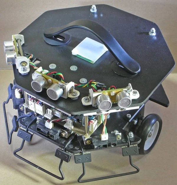
Step 1: The Basic Platform

An example of how to build up a very simple robotic platform with components and parts easy to find everywhere, without the needs of professional tools or equipment, and without a special skill on mechanical works.
The size of the base allows its use in many different categories of robotic contests: Explorer, Line Follower, Can Collector, etc.

Step 2: What We Want to Obtain? and How?

This robot, as most of the robots built by hobbysts, is based on a differential steering system, allowing us to know the position coordinates of the robot at any given moment, simply knowing the space covered by each wheel periodically with enough precision.
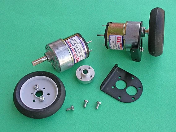
This dead reckoning navigation system is affected by cumulative error; the measuring precision must be high to ensure a small error circle after a long path. So, after some good results with homemade encoders, I decided to use something better: a couple of 12V-200 rpm geared motors, connected to a couple of 300 Count Per Revolution (cpr) encoders, both available at many Internet robotics shops.

Basic principles
To catch all the pulses generated by the 300 cpr encoder on a 3000 rpm motor in 4x decoding method (120 kHz), we need dedicated hardware for each encoder (QEI = Quadrature Encoder Interface). After some experimenting with a double PIC18F2431, I determined that the correct upgrade is to a dsPIC. At the beginnig they were two dsPIC30F4012 motor controllers to control wheels position and speed, to perform odometry and to provide data of the two motors to a dsPIC30F3013. This general purpose DSC is powerful enough to get data, do some trigonometry in order to calculate position coordinates, and store data related to the path covered in order to obtain a map of the field, all at a very high rate.

When the board and the programs were almost completed, Microchip brought out a new, powerful 28-pin SPDIP in the dsPIC33F series for both motor controller (MC) and general-purpose (GP) versions. They are significantly faster than the dsPIC30F, they have a lot more available program memory and RAM (useful for field mapping), they require less power (good for a battery-operated robot), and their DMA capabilities simplify many I/O operations.
Most importantly, these are the first Microchip motor controllers with two QEIs on the same chip. Let’s start a new port again! The logical block diagram is similar to the one for the previous board , but the hardware and software are much simpler since I can use one DSC only insted of three . There is no need for an high-speed communication between the supervisor and motor controllers to exchange navigation parameters. Every process is simple to synchronize because it’s on the same chip. The peripheral pin select capability of the dsPIC33F series further simplifies the PCB, enabling an internal connection of peripherals and a greater flexibility .

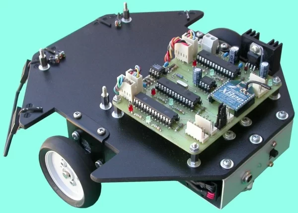
This brings us to the “dsPIC based Navigation Control board” or dsNavCon for short. This board is designed as a part of a more complex system. In a complete explorer robot, other boards will control sound, light, gas sensors, as well as bumpers and ultrasonic range finders to find targets and avoid obstacles.

As a standalone board, dsNavCon can also be used for a simple “line follower” robot, something more complex like a robot for an odometry and dead-reckoning contest, or a so called “can can robot” (for can collecting competitions). There still is plenty of free program memory to add code for such tasks. With minor or no changes in software, it can also be used standalone for a remote controlled vehicle, using the bidirectional RF modem with some kind of smart remote control. This remote control can send complex commands like “move FWD 1m,” “turn 15° left,” “run FWD at 50 cm/s,” “go to X,Y coordinates,” or something similar.

The board and the robot too, are designed to be made by anyone at home without professional tools and equipment.

Step 3: The Open Source Hardware

Block Diagram
The navigation control subsystem is composed of the dsNav as the “smart” board of the system and a L298-based dual H-bridge board to control the geared 12V motors (Hsiang Neng HN-GH12-1634TR). The motion feedback comes from a couple of 300 cpr encoders (US digital e4p-300-079-ht).
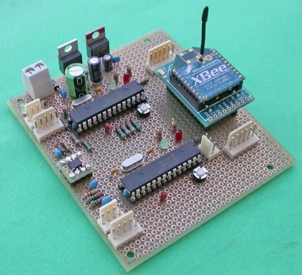
The communication with the external world is performed through the two UART serial interfaces; one for telemetry and the other to get data from sensors board. The XBee module can be connected to UART1 or UART2 through JP1 and JP2 jumpers. J1 and J16 sockets are available for other kind of connections. COMM1 port (J16) can also be used for an I2C communication thanks to the peripheral pin select capability of the dsPIC33F series.

The original schematic diagram in Eagle format can be found here:
http://www.guiott.com/Rino/dsNavCon33/dsNavCon33_Eagle_project/DsPid33sch.zip

As you can see the schematic is so simple that it can be implemented on a perfboard as I did. If you don’t want to use this system and don’t want to realize your own PCB, a commercial board based on my original work and fully compatible with my open source software is available at: http://www.robot-italy.com/product_info.php?products_id=1564

Step 4: The Open Source Software

The software is developed with MPLAB® free IDE and written with MPLAB® C30 compiler (even in a free or student version), both (of course) by Microchip:
http://www.microchip.com/stellent/idcplg?IdcService=SS_GET_PAGE&nodeId=81

The whole project is available as open source at Google Code
http://code.google.com/p/dspid33/
Please refer there for the latest version, comment, descriptions, etc.
The program is described step by step inside the code. In order to have a high level of commenting and a more readable code, at every significant point there is a number in brackets (e.g.: [7]) as a reference to an external file (i.e.: descrEng.txt) in the MPLAB project.

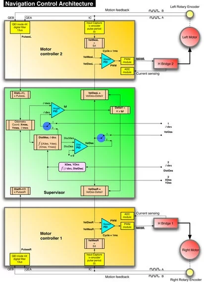
The diagram shows the overall architecture of the control procedures of dsNav board and the navigation strategies applied at the basis of the project.
The motor controllers can be seen as black boxes that take care of the speed of the wheels. The supervisor part of the program sends them the reference speed (VeldDesX: desired velocity). The Input Capture modules of the microcontroller get pulses from the encoders connected to the motor axis and derive the rotational speed of the motors (VelMesX: measured velocity). Combining every 1ms this values in the PID control “Speed PID” we obtain the right PWM value to keep the desired speed of each single wheel.
The QEI (Quadrature Encoder Interface) modules get both the A and B pulses from the encoders and give back to the supervisor function the traveling direction and the number of pulses in 4x mode (counting the rising and falling edges of signal A and signal B: 2 x 2 = 4) .
Multiplying the number of pulses by a K that indicates the space traveled for each single encoder pulse, we obtain the distance traveled by right and left wheels every 10ms. The supervisor combines this traveling informations and applies the dead reckoning procedure in order to obtain the measured position coordinates of the bot: Xmes, Ymes, θMes (orientation angle).

The supervisor receives navigation command from outside by serial interface (telemetry) .
Different strategies can be applied:
A – travel at a given speed in a given direction (VelDes, θDes).
B – travel toward a given point with coordinates XDes, YDes.
C – travel for a given distance in a given direction (DistDes, θDes).

Mode A : with the “logical control switches” in position 1, only the PID control “Angle PID” is used by the supervisor functions. This one combines the desired angle θDes with the measured angle θMes calculated by odometry procedure, in order to obtain the value of the rotation angular speed ω of the vehicle around its vertical axis, needed to correct the orientation error.
The value of DeltaV is proportional to ω. It’s added to VelDes to obtain the speed of the left wheel and subtracted to VelDes to obtain the speed of the right wheel, in order to keep the heading corresponding to θDes value, while the center of the robot is still traveling at VelDes speed.

Mode B : with the “logical control switches” in position 2, the desired speed VelDes is calculated by the PID control “Dist PID” and it is used as in mode A. The measured input for this PID (DistMes) is computed as a function of the current coordinates and the destination coordinates. The desired orientation angle θDes also comes from the same procedure and it’s used as reference input for “Angle PID”. The reference input for “Dist PID” is 0, meaning that the destination is reached. With ω and VelDes available, the speed control of the wheels runs as in mode A.

Mode C : with the “logical control switches” in position 2, the destination cordinates Xdes, Ydes are computed once at the beginning as a function of input parameters DistDes, θDes. After that everything goes as in mode B

Step 5: Details of Software: Speed Control and Other Basic Functions

The program is full interrupt driven . At the startup, after initialization, the program enters in a very simple main-loop, acting as a state machine. In the main-loop, the program checks flags enabled by external events, and it enters in the relative state according to their values.

Since it’s a kind of a very simple cooperative “Real Time Operating System ,” each routine has to be executed in the shortest possible time, freeing the system up to take care of the very frequent interrupts.
There are no “wait until” and no delays in the code. Whenever possible interrupts are used, in particular for slow operations like transmission or reception of strings of characters. UART communication takes the advantege of the DMA capabilities of the dsPIC33F to save CPU time doing all the “dirty” job in hardware.

Peripherals used on dsPIC33FJ128MC802:
– QEIs to calculate the traveled path.
– Input Capture (IC) to calculate speed.
– A/D converters to read motor current.
– Enhanced PWMs to drive the motors.
– UARTs to communicate with the external world

QEI modules are used to know how much the wheels have traveled and in which direction. This value is algebraically cumulated in a variable every 1ms and sent to the supervisor functions at its request. After the value is sent, the variables are reset.

Speed is measured at every encoder’s pulse as described below. Every 1ms it calculates the mean speed by averaging samples, executes PID algorithm, and corrects the motor speed accordingly to its result, changing PWM duty cycle. For a detailed description of C30 PID library application, see Microchip Code Example: CE019 – Using Proportional Integral Derivative (PID) controllers in Closed-loop Control Systems. http://ww1.microchip.com/downloads/en/DeviceDoc/CE019_PID.zip

Speed variations of the motors are executed smoothly, accelerating or decelerating with a rising or falling slanted ramp, in order to avoid heavy mechanical strain and wheel slippage that could cause errors in odometry. Deceleration is faster then acceleration to avoid bumps with obstacles during braking.

IC , input capture modules are used to measure the time elapsed between two pulses generated by the encoder,s meaning when the wheels traveled for a well-known fixed amount of space (constant SPACE_ENC ). Connected in parallel to QEA (internally to the DSC thanks to the Peripheral Pin Select capabilities of the dsPIC33F), they capture elapsed time on rising edge of encoders signals. TIMER2 is used in free-running mode. At each IC interrupt, TMR2’s current value is stored and its previous value is subtracted from it; this is the pulse period. Then the current value becomes the previous value, awaiting the next interrupt. TMR2’s flag has to be checked to know if an overflow happened in the16-bit register. If yes, the difference between 0xFFFF and the previous sample has to be added to the current value. Samples are algebraically added in IcPeriod variable according to _UPDN bit, to determine also the speed direction. This is one of the suggested methods in Microchip application note AN545 .
The variable IcIndx contains the number of samples added in IcPeriod .
Every 1ms the mean speed is calculated as V=Space/Time
where Space=SPACE_ENC•IcIndx
(= space covered in one encoder pulse • number of pulses)
and Time=TCY•IcPeriod
(= single TMR period • summation of periods occurred).
Single_TMR_period=TCY=1/FCY (clock frequency).
So V=Kvel•(IcIndx/IcPeriod)
where Kvel=SPACE_ENC•FCY to have speed in m/s.
Shifting left 15 bits Kvel const (KvelLong=Kvel<<15 ) the velocity is calculated already in fractional format (also if only integer variables are used) ready to be used in PID routine. See “descrEng.txt” file in MPLAB project for a more detailed description.

A/D converters continuously measure motors current, storing values in the 16 positions ADCBUF buffers. When buffers are full, an interrupt occurs and an average value is calculated approximately every 1ms.

UARTs are used to receive commands from outside and to send back the results of the measurements. The communication portion of the program runs as a state machine. Status variables are used to execute actions in sequence. Very simple and fast Interrupt Service Routines (ISR) get or put every single byte from or to a buffer, and set the right flags to let the proper function to be executed.

If any kind of error occurs during receiving (UART, checksum, parsing errors), the status variable is set to a negative number and the red led is powered up to communicate externally this fault condition. See “descrEng.txt” file in MPLAB project for a complete list of possible errors.

The protocol used for the handshake is physical layer independent , and can be used with the I2C or RS485 bus as well to communicate.
The first layer is controlled by dsPIC peripheral interface. Frame or overrun errors (UART) or collisions (I2C) are detected by hardware, setting the appropriate flag.
The second layer is handled by ISR routines. They fill the RX buffer with the bytes received from the interfaces. They also detect buffer overflow and command overrun.
UartRx or UartRx2 functions manage the third layer . As already described (see also flow charts) these routines act as a state machine, getting bytes from the buffer and decoding the command string.
The bytes are exchanged between second and third layers (ISR and UartRx function) through a circular buffer. ISR receives a byte, stores it in an array and increments a pointer to the array, if the pointer reaches the end of the array it is restarted to the beginning. The UartRx function has its own pointer to read the same array, incremented (in a circular way too) as soon as the byte is decoded in the current RX status. Main loop calls the UartRx function whenever the “in” pointer differs from “out” pointer.

Each command packet is composed by:
0 – Header @
1 – ID 0-9 ASCII
2 – Cmd A-Z ASCII
3 – CmdLen N = 1-MAX_RX_BUFF # of bytes following (checksum included)
4 – Data …
…
N-1 – Data
N – Checksum 0-255 obtained by simply adding up in an 8 bits variable, all bytes composing the message (checksum itself excluded).

This layer controls timeout and checksum errors, as well as packet consistency (correct header, correct length). If everything is ok it enables Parser routine (fourth layer ) to decode the message and to execute the action required. This routine sets the appropriate error flag if the message code received is not known.

TMR1 generates a 1000 Hz timing clock – the heartbeat of the program. On each TMR1’s interrupt, internal timers are updated, the watchdog is cleared, and a flag is set to enable the function that asks for the traveled space value. Every 10ms “All_Parameters_Ask” function (speed, position, current) is enabled.

Step 6: Details of Software: Odometry and Field Mapping = Where Am I?

Optimization of the general algorithm for a use in a DSC or MCU based system
Once we have the information about the distance traveled by each wheel in a discrete-time update (odometry), we can estimate the position coordinates of the robot with the same periodicity without any external reference (dead reckoning).
Some theoretical background regarding dead reckoning by odometry can be found in the book by Johann Borenstein:
“Where Am I? – Sensors And Methods For Mobile Robot Positioning”
and on the following web pages:
http://www.seattlerobotics.org/encoder/200010/dead_reckoning_article.html
The mathematical background and a deep explanation of the general method used, can be found on G.W. Lucas’ paper A Tutorial and Elementary Trajectory Model for the Differential Steering System of Robot Wheel Actuators, available on Internet:
http://rossum.sourceforge.net/papers/DiffSteer/DiffSteer.html

Some simplified algorithms can be found in that same documentation too, so it’s possible to obtain the correct compromise between precision and speed of elaboration, using the mathematic (trigonometric) capability of dsPIC33F series.
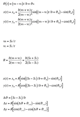
A description of the maths used to compute the position can be found in the pictures attached to this step. The first one shows the meaning of the symbols, the second one shows the formulas used with those symbols. Clicking the boxes next to each computational step a brief description is shown.

At the end we know how much the robot moved in that time interval as a delta of the orientation, a delta on X axis and a delta on Y axis in the carthesian reference field.
Cumulating each delta-value in its own variable we know the current coordinates (position and orientation) of the platform.

In order to avoid computational errors (divide by zero) and waste of the controller time, a check has to be done in advance on both Sr and Sl variables. Defining a quasi-zero value that takes care of minimal mechanical and computational approximations we can simplify the formulas if the robot is traveling in a straight line (the space covered by the right wheel is almost the same as the space traveled by the left wheel) or if it’s pivoting around its vertical axis (the space covered by the right wheel is almost the same as the space traveled by the left wheel but in a opposite direction), as detailed in the flow chart shown in the last picture.

This video shows an example of which precision we can obtain:
http://www.youtube.com/watch?v=d7KZDPJW5n8

Field mapping
With data computed by previous functions a field mapping is performed.
Every Xms, after the current position elaboration, a field mapping is performed dividing the unknown field in a 10 x 10cm cells grid. Defining a maximum field dimension of 5 x 5m, we obtain a 50 x 50 = 2500 cells matrix. Each cell is defined with a nibble, with a total memory occupation of 1250 Bytes. Sixteen different values can be assigned to each cell:
n = 00 unknown cell
n = 01 – 10 cell visited n times
n = 11 obstacle found
n = 12 gas target found
n = 13 light target found
n = 14 sound target found

The robot can start from any position in the field; these will be the reference coordinates (0,0) in its reference system.
Field mapping is useful to find the best exploring strategy in an unknown field. The robot can direct itself to the less explored portion of the field (lower “n” value), can save time by not stopping twice in an already discovered target, can find the best path to reach a given coordinate, and more.

Step 7: Remote Console

This is the application that remotely controls the dsNavCon board from a Mac/PC via serial communication through a couple of XBee devices as described in the block diagram.
In order to be easy to develope and good to run in any operating system, it’s written with Processing language:
http://www.processing.org/

The source code for this program too is available as open source at Google Code:
http://code.google.com/p/dsnavconconsole/

With the main panel (first pictures) we can perform telemetry by looking on the grid the path followed by the robot (as estimated by odometry) in a configurable size field and some other important values read on the dsNav .
The gauges show the measured values:
– MesSpeed in a +/- 500 mm/s range, the mean value of the two wheel’s speed (the speed of the center of the platform).
– Measured Current in mA (the sum of the current from the two motors).
– Measured Angle, as extimated by odometry.

Other panels are used to configure the parameters of the robot and to store into the robot a defined path to follow  (if needed). An important panel, at least during development of the robot, is the detail panel (second picture) that shows the speed of each wheel in real time, very useful for the calibration of all the parameters.
The central grid view can be switched with the view of a webcam to control, even by view, the path  the robot is following.

A practical example of usage for this console is shown in this video:
http://www.youtube.com/watch?v=OPiaMkCJ-r0

Source: How to Build a Self Navigating Robot