Summary of Third version of homemade 6 GHz FMCW radar
The author improves a budget FMCW radar by addressing noisy power supplies, unsynchronized clocks, and insufficient microcontroller processing. Key upgrades include adding linear regulators for clean power, synchronizing ADC and PLL clocks to reduce phase noise, and utilizing an FPGA for digital signal processing. A second receiver antenna is added for direction finding. The article details link budget calculations, receiver dynamic range considerations involving LNAs and mixers, and noise floor analysis using FFT processing gain to determine maximum detection ranges for various targets.
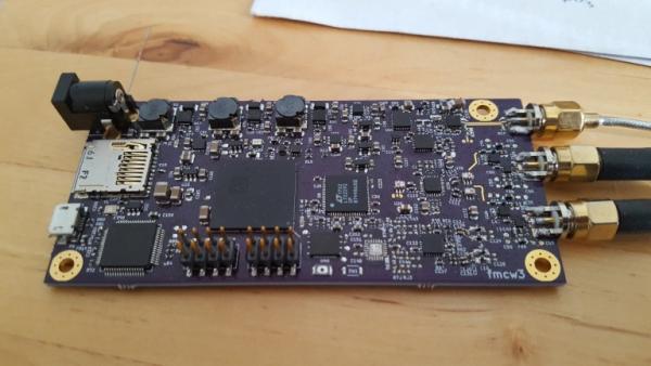
Parts used in the Improved FMCW Radar:
- Buck converters
- Linear regulator
- ADC sampling clock
- PLL reference clock
- Microcontroller
- FPGA
- Second receiver antenna
- Horn antennas
- Patch antennas
- LTC2292 ADC
- Low noise amplifier (LNA)
- Mixer
- IF amplifier
- Op-amps
Introduction
Previously I made a simple frequency-modulated continuous-wave (FMCW) radar that was able to detect distance of a human sized object to 100 m. It worked, but as it was made with minimal budget and there was a lot of room for improvement.
FMCW radar working principle
FMCW radar block diagram
If you have read my previous articles you should know how FMCW radar works, but for completeness sake short explanation is given below:
Frequency Modulated Continuous Wave (FMCW) radar works by transmitting a chirp which frequency changes linearly with time. This chirp is then radiated with the antenna, reflected from the target and is received by the receiving antenna. On the reception side the received signal that was delayed and undelayed copy of the transmitted chirp are mixed (multiplied) together. The output of the mixer are two sine waves that have frequencies of sum and difference of the waveforms. The frequencies of the received signals are almost the same and the sum waveform has frequency of about two times of the original signal and is filtered out, but the difference waveform has frequency in kHz to few MHz range. The difference frequency is dependent on the delay of the received reflection signal making it possible to determine the delay of the reflected signal. The electromagnetic waves travel at speed of light which allows converting the delay to distance accurately. When there are several targets the output signal is sum of different frequencies and the distances to the targets can be recovered efficiently with Fourier transform.
Issues with the previous version
The biggest issue with the previous version was noisy power supplies causing spurs in the received signal, ADC sampling clock not being locked to PLL reference clock and microcontroller being too slow.
To save money I had chosen to use two buck converters to power all the digital and analog components. Even though I chose the switching frequency of the converters to be above the IF frequency, there ended up being some spurs also at lower frequencies. Adding capacitance and swapping the inductors for better shielded ones helped the problem but didn’t completely solve it. The proper fix is to add linear regulator after the buck converters to clean up the switching noise.
The problem with separate clocks for ADC and PLL caused the sampling interval of the ADC to vary between separate sweeps. The maximum offset was only +- half a sample and it wasn’t a big issue when only doing range measurements. However when trying to measure heartbeat and respiratory rate the added phase noise from the varying sampling interval caused some noise in the measurements. Noisy power supplies also degraded the phase noise performance. The fix for this one is pretty easy: Use the same clock for both ADC and PLL.
The microcontroller I was using was pretty powerful compared to the cheapest 8-bit microcontrollers, but it was hopelessly underpowered to do any kind of digital signal processing. All of processing power and internal memory was spent in getting the samples from ADC to PC through USB fast enough. Sampling speed of the ADC was 10 MHz and because of lack of DSP resources every sample needed to be transferred to PC. Even the samples between the sweeps that didn’t have any useful data were transferred to PC only to be discarded later. With more resources it would have been possible to do digital filtering, lower the sampling speed and only transfer the useful samples.
Microcontrollers don’t really have enough processing power to do any kind of non-trivial filtering. For example a 100 tap FIR filter requires 100 multiplications and 100 additions for every sample. Even if the multiplication could be done in one clock cycle the maximum sample rate is too low to be useful. The microcontroller should also have enough processing power to transfer ADC samples and do communication and other logic. FPGA works much better for DSP as the operations can be done in parallel.
The last improvement is adding a second receiver antenna. When there are more than one receiver antenna it is possible to determine the direction of arrival of the received signal. If the return signal arrives in angle it is received at different antennas at different times. The different arrival time causes a phase shift in the IF signal which can be used to determine the direction.
Link budget
Since I’m not changing the transmitter, the maximum range performance should be pretty identical to the last version when using the same horn antennas. When smaller patch antennas are used as receiver antennas the range is going to decrease because the gain and efficiency of the patch antennas is smaller.
The maximum range to detect a target can be calculated using the radar equation:
where PtPt is the transmitted power, GG is gain of the antennas, λλ is wavelength, σσ is the radar cross section of the target and PminPmin is the minimum detectable signal power.
Most of the values are easy to determine, but the minimum detectable power can be tricky. Clearly the minimum power that can be detected depends on the noise level of the receiver. Noise at the receiver input is RF thermal noise, which can be calculated with kTBFkTBF, where kk is the Boltzmann constant, TT is noise temperature, BB is noise bandwidth and FF is the receiver noise figure.
Determining the correct noise bandwidth to be used is critical and easy to get wrong. Noise bandwidth is clearly smaller than the sweep bandwidth since the IF filter filters most of the RF noise out. IF filter bandwidth determines the noise power that makes it to the ADC, but that is not the noise bandwidth to be used since some of the noise can be clearly filtered out after taking the FFT. When FFT is taken of the IF signal the total RF noise is split equally to each FFT bin. Bandwidth of one FFT bin is the noise bandwidth of the receiver and the bandwidth that should be used in the calculation. Bandwidth of one FFT bin depends only of the lenght of the FFT. With FMCW radar FFT length equals length of one sweep, tsts and bandwidth of one FFT bin is 1/ts1/ts.
With sweep length of 1 ms and noise figure of 6 dB the RF noise floor at the receiver input is -138 dBm. For the signal to be detectable it should be some amount more powerful than the noise. Using 20 dB for the required signal-to-noise ratio gives minimum detectable signal of -118 dBm.
| Variable | Explanation | Value |
|---|---|---|
| PtPt | Transmitted power | 15 dBm |
| GG | Gain of antennas | 13 dBm |
| λλ | Wavelength | 5.2 cm |
| σσ | Target radar cross-section | 1 m² |
Plugging the values above to the radar equation the maximum range that radar can see a human sized 1 m² cross-section target can be solved to be 320 m. The target size does have a big effect, for example a bird sized target with cross-section of 0.01 m² can be detected only below 102 m. The transmitted power in the table is somewhat pessimistic to include losses from antennas, cables and PCB.
This would be correct for radar looking at air, but when the radar antennas are looking at a low angle there is going to be problem with clutter that can decrease the SNR. When angle of the antennas is low and the radar is on a flat ground there is going to be returns from the ground from basically every range. Returns from other objects such as trees, buildings and other objects can also overlap the target signal decreasing the signal to noise ratio.
Receiver design
Simplified radar block diagram.
The previous range calculation assumed that the receiver has sufficient dynamic range to detect the RF noise floor, linearity is good enough. Care should be taken especially with the dynamic range of the receiver since reflections from targets near the antennas are going to have much larger power than the noise floor and the receiver should be able to resolve both returns at the same time.
Noise figure of the receiver should be kept as low as possible which can be done by choosing a low noise amplifier with low noise figure and high gain. Higher the gain of the LNA is the smaller the noise contributions of the following stages. A drawback of having high gain is that the input compression point is lowered as either the LNA output stage, mixer or IF amplifier starts to saturate earlier due to higher output power of the high gain LNA. If the input compression point is too low receiver can saturate just from the leakage power between the transmission and receiver antennas. In saturation the receiver doesn’t work linearly anymore and many harmonics are generated that are detected as false targets. It’s very important to avoid saturating the receiver and this is one of the major issues when using single antenna that is shared between transmitter and receiver. Radar with a low input compression point has higher minimum detection distance below which the returns from the targets saturate the receiver. Choosing the LNA gain ends up being a compromise between noise and input compression point.
It’s important to also take into account the noise figure of the low frequency amplifier driving the ADC and noise floor of the ADC. Op-amps typically can’t be analyzed using noise figure because ports aren’t matched to 50 ohms. The right way is to convert the RF noise to V/Hz−−−√Hz. However comparing the input noise voltage density of the op-amp to noise voltage density of 50 ohm resistor gives a close enough value for hand calculations. Usually op-amps have quite high noise figure due to the resistors used to set the gain. NF of ten to twenty dB is usually a good guess.
ADC has quantization noise and input noise that results in limited dynamic range. Datasheet of the ADC lists the SNR which is calculated by measuring a maximum amplitude sine wave, taking FFT and then dividing the signal power by noise power in all other FFT bins. The dynamic range can be increased with oversampling and filtering. The noise floor after taking the FFT is considerably better than the SNR number listed in the datasheet because noise at different frequencies can be separated.
The dynamic range of the ADC with the FFT processing gain can be calculated with:
where SNR is the SNR of the ADC listed in the datasheet, fsfs is the sampling frequency and tsts is sweep length. LTC2292 ADC that I used has listed SNR of 71.3 dB and sampling frequency is 40 MHz. This gives ADC dynamic range of 117 dB with 1 ms sweep.
To make sure that the ADC doesn’t limit the system performance the RF noise floor after the ADC should be above the ADC noise floor. The input referred RF noise power at the LNA input is kTBF=kTF/tskTBF=kTF/ts. This is amplified by the LNA and mixer by GLNAGmixerGLNAGmixer. After the mixer the RMS output voltage can be calculated as V=ZloadP−−−−−√V=ZloadP, where ZloadZload is the mixer output impedance (200 Ω on the mixer I’m using). This voltage is amplified by the IF amplifier by GIFGIF. Next the RMS voltage should be converted to peak-to-peak value by multiplying by 22–√22 and then referenced to maximum ADC voltage range. Finally by taking 20log1020log10 we will get the noise floor in dBFs units (relative to ADC maximum input signal). Putting it all together in one equation gives:
| Variable | Explanation | Value |
|---|---|---|
| VrefVref | ADC maximum peak-to-peak voltage | 2 V |
| GIFGIF | IF amplifier gain | 20 dB |
| GLNAGLNA | LNA gain | 20 dB |
| GmixerGmixer | Mixer power gain | 0 dB |
| kk | Boltzmann constant | 1.38064852×10⁻²³ m2 kg s-2 K-1 |
| TT | Noise temperature | 290 K |
| ZloadZload | Mixer output impedance | 200 Ω |
| FF | Receiver noise figure | 6 dB |
| tsts | Sweep length | 1 ms |
Read More: Third version of homemade 6 GHz FMCW radar
- What causes spurs in the received signal?
Noisy power supplies from buck converters cause spurs in the received signal. - How can you fix the issue with varying sampling intervals?
Use the same clock for both the ADC and the PLL to eliminate phase noise caused by separate clocks. - Why is the microcontroller considered underpowered?
The microcontroller lacks sufficient resources for digital signal processing like filtering and must transfer every sample to the PC. - What component works better for DSP than a microcontroller?
An FPGA works much better for DSP because operations can be done in parallel. - Does adding a second receiver antenna help?
Yes, it allows determining the direction of arrival by analyzing phase shifts between antennas. - How does target size affect detection range?
A smaller target like a bird with a 0.01 m² cross-section can only be detected below 102 m compared to 320 m for a human. - What determines the minimum detectable signal power?
The minimum detectable power depends on the noise level of the receiver calculated via kTBF. - What happens if the receiver input compression point is too low?
The receiver may saturate from leakage power, generating harmonics that are detected as false targets. - How is the noise bandwidth determined after taking an FFT?
The bandwidth of one FFT bin equals the sweep length inverse and serves as the noise bandwidth. - Can patch antennas replace horn antennas without issues?
Using smaller patch antennas decreases the range because their gain and efficiency are smaller than horn antennas.