Summary of FFTs and oscilloscopes: A practical guide
The FFT (Fast Fourier Transform) adds frequency-domain analysis to oscilloscopes by computing the Discrete Fourier Transform efficiently. Modern scopes include FFTs from hobby to lab models. Using an FFT reveals signal characteristics like bandwidth and frequency distribution that are hard to see in the time domain; for example, an amplitude-modulated, linearly swept RF carrier whose time view hides its 4.7 MHz bandwidth is clear in the FFT spectrum. The guide focuses on practical setup and use rather than FFT math.
Parts used in the FFTs and oscilloscopes project:
- Digital oscilloscope with FFT capability
- RF carrier source (signal generator)
- Amplitude modulation source (pulse or waveform generator)
- Trapezoidal pulse generator (for modulation)
- Probes or RF cabling
- Cursors or marker tools (on the oscilloscope)
The FFT (Fast Fourier Transform) first appeared when microprocessors entered commercial design in the 1970s. Today almost every oscilloscope from high-priced laboratory models to the lowest-priced hobby models offer FFT analysis. The FFT is a powerful tool, but using it effectively requires some study. I’ll show you how to set up and use the FFT effectively. We’ll skip the technical description of the FFT, because its already implemented in the instruments. Instead I’ll focus on the practical aspect of using this great tool.
The FFT is an algorithm that reduces the calculation time of the DFT (Discrete Fourier Transform), an analysis tool that lets you view acquired time domain (amplitude vs. time) data in the frequency domain (amplitude and phase vs. frequency). In essence, the FFT adds spectrum analysis to a digital oscilloscope.
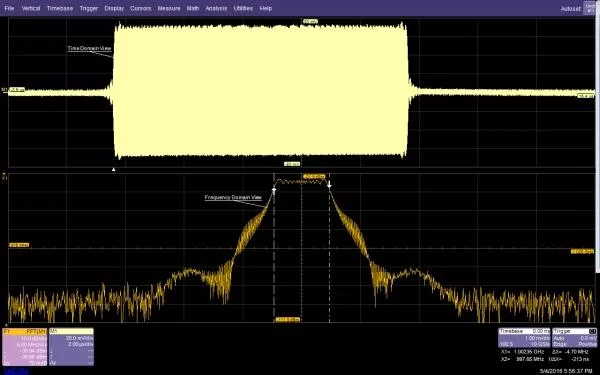
If you look at upper trace in Figure 1, you’ll see an amplitude-modulated carrier that uses a trapezoidal pulse as the modulation function. If you look at the time-domain view in Fig. 1 and I ask you to tell me the bandwidth of the signal, you’d have a hard time. But take the FFT of this signal and you get another point of view. The signal has a linearly swept frequency and the bandwidth, marked by the cursors, is 4.7 MHz. That’s how the FFT adds to the capability of the oscilloscope, it provides another point of view for the same data.
Figure 1. The time domain view in the top grid shows a pulse modulated RF carrier while the frequency domain view in the lower grid shows a uniform distribution of the carrier frequency between 997 MHz and 1002 MHz.
Read more: FFTs and oscilloscopes: A practical guide
- What does the FFT add to a digital oscilloscope?
The FFT provides frequency-domain analysis (amplitude and phase vs. frequency) of time-domain data. - Can every oscilloscope perform an FFT?
Yes, almost every oscilloscope from high-priced laboratory models to low-priced hobby models offers FFT analysis. - How does the FFT help with bandwidth measurement?
The FFT reveals the frequency distribution and allows cursors to mark and measure bandwidth, which may be difficult to see in the time domain. - Does the article explain FFT mathematics?
No, the article skips the technical description of the FFT and focuses on practical usage and setup. - What example signal is used to demonstrate FFT benefits?
An amplitude-modulated RF carrier using a trapezoidal pulse as the modulation function is used as the example. - How is a linearly swept carrier shown in the FFT?
The FFT shows a uniform distribution of the carrier frequency across the swept range, revealing the bandwidth between frequency limits. - What bandwidth is identified in the example?
The example identifies a bandwidth of 4.7 MHz using the FFT and cursors.