ECE 4760 Final Project: 3d lidar imaging system

Introduction

The goal of this final project was to create a lidar 3d imaging system while on a limited budget. This is a system which takes many distance readings while pointing at many different angles. These distance readings are then converted into cartesian points and then plotted onto a graph. By plotting thousands of points, a three-dimensional image of the scene the system is pointed at is created.

The motivation for this project was to create a 3d imaging system which can be used for data collection by the Autonomous Systems Lab without having to buy a very large professional system. There are many other 3d imaging systems available, but they are generally expensive, costing several thousand dollars. The result of this is only having a 3d lidar imaging system in very large projects, such as for autonomous driving. There are many projects which could use 3d image data which simply do not have the several thousand dollars to buy the 3d imaging system. This project is designed to show that with a budget of around 200 dollars, a 3d lidar imaging system can be made which produces useful data.

High Level Design

Rationale

The idea for creating a 3d lidar imaging system came to me because of a past internship at a company developing a lidar sensor. The lidar sensor being developed created beautiful images and had an extremely long range, but the system was very expensive. The concept behind the 3d lidar system is not too complicated; you simply need to move a distance sensor through a scan pattern and collect data. Collecting this data at a fast rate while maintaining data accuracy, however, is a very difficult task. This is why professional systems are expensive; a 3d lidar imaging system requires very high-precision and well-tuned components. If, however, you settle for a less accurate and slower system, it becomes possible to create a 3d lidar image while under the constraints of a much tighter budget.

Logical structure

The three main components of this system are 2 servos, a lidar distance sensor and a PIC32 microcontroller. At a high level, this system works by directing where the lidar sensor is pointing by mounting this sensor onto two servos, one determining the azimuth angle and one determining the altitude angle. These servos are being controlled by the PIC32 so that they each move in a triangle wave pattern with each servo moving at a different frequency; this creates a scan pattern. Finally, analog feedback data from the servos is fed into the PIC32 to provide accurate position data of the servos. The culmination of all this is a lidar distance sensor which is moving through a scan pattern and constantly measuring distances, and all of these distance measurements are associated with both an azimuth and an altitude angle. These three measurements can then be converted to cartesian coordinates and recorded. After several thousand of these points are recorded, the result is a 3d image.

Background Math

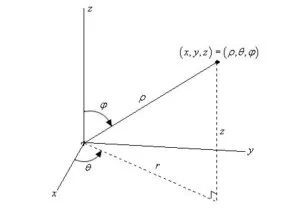
Most of the work being done by the microcontroller is either collecting data or sending out a PWM signal to control the servos. The only real computation being done by the PIC32 is the conversion from the raw data collected into cartesian points, and the math behind this conversion is quite simple. The data collected can be thought of as spherical coordinates; the lidar distance data is the radial distance and the two servo feedback values are the azimuth and radial angles. The math to convert from the raw data to the cartesian points, then, is simply the formulae used to convert from spherical coordinates to cartesian coordinates.

Hardware Software Tradeoffs

For this project, there were not too many design decisions which came down to either hardware or software; most of the components had to be one or the other. For example, the power isolation cannot be done in software, and the PWM signal controlling the servos cannot be done in hardware. One component where there was a decision, however, was the filter for the analog feedback signal coming from the servos. This analog feedback is both noisy and does not fully utilize the range between 0 and 3.3V. That is why I decided to use a combination of hardware and software to filter the signal. The hardware portion of the filter was a differential amplifier; this increased the range of the analog feedback voltage before going into the ADC. By performing this step in hardware, I was able to get a wide range of ADC units when reading the feedback without discretizing the feedback. The software portion was a Kalman filter. This filter helped to reduce the noise coming from the analog feedback signal so that a more precise angle could be recorded. The benefit of this type of filtering was the ease of changing the filtering parameters. The Kalman filter is a relatively cheap computation, and it is very easy to change the one parameter it uses in software. This allowed me to test many different values for this parameter without much work. Had I tried to perform some type of filtering in hardware, there would have been a lot more work when tuning the filter to give the best output as a the physical circuit would have to be changed for every iteration of the filter.

Standards and Copyrights

The laser being used falls under the laser classification Class 1 in IEEE standard. This means that the laser is safe to view even with instruments. As for copyrights, no idea or design in this project is protected by copyright or trademark.

Software and Hardware Design

Software Overview

The software portion of this project consisted of three main parts: controlling the servos, collecting data from the servos and the lidar sensor, and performing analysis on this data before sending the data to either the TFT display or over UART. Additionally, there was also a simple heartbeat light used on the board to show that the system was in operation.

Controlling Servos

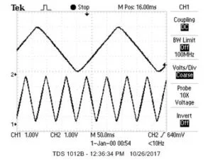
The servos used take as an input a PWM control signal. By connecting a PWM signal of a certain length, the servos will go to a certain position. This PWM signal needed to have a period of at least 20ms and the PWM on range needed to be between around 10% and 30% of the cycle. The challenge for this project was to create a triangle wave with these PWM signals. To do this, an ISR was used which was hooked up to an internal timer set to trigger the ISR at 125Hz. Also, two output compares were initialized and hooked up to a timer which had a period of 40ms. Every time the ISR was called, the value for the number of timer ticks the PWM should be high was recalculated and sent to these output compares. These values, pwm_on_times, were calculated by simply increasing or decreasing the two values linearly until they reached a min or a max value, and then they started going back. The result of this was a PWM which was linearly increasing and decreasing in a triangle pattern. The frequency of this triangle pattern could be easily set by changing the increment value for the pwm_on_times, and the max and min of the pwm_on_times could be set by changing when to change from incrementing to decrementing or vice versa. Since the azimuth and the altitude servos needed to move at different frequencies, the two pwm_on_times were incremented and decremetented at different rates from one another. Below is the output of these PWM signals after going through a low-pass filter. The voltage goes from 0 to 3.3V because this waveform was captured early in the building of the project, but the wave form shape and the difference in frequencies between the two servo control signals can be seen.

Capturing Data

Capturing data was also done in an ISR, though this time the ISR was triggered by a hardware event. The lidar sensor works by outputting a PWM signal with a time high equal to 10 microseconds per centimeter. By setting the lidar to constantly take distance measurements, the result is a stream of PWM signals with varying lengths correlating to different distance measurements. To capture this PWM length, two input captures connected to a free running clock with a tick rate of 5MHz was used. A 5MHz clock was used to be able to capture the full PWM length without overrunning too often. One wire connected to the lidar output signal was connected to the first input capture, and this input capture was set to trigger an ISR on every rising edge of the output signal. On the rising edge, the timer value recorded by the input capture was read and saved. The output signal of the lidar was also connected to the second input capture, and this input capture was set to trigger an ISR on every falling edge of the lidar output signal. On the falling edge of the output, the timer captured by the second input capture was read. The system now has 2 input capture times, so the lidar distance measured can be calculated later using the difference of the two. After first checking to see that the falling edge is larger than the rising edge to ignore capturing time events during a timer overrun, the values were subtracted from each other and put into an array which acted like a bounded buffer. Accordingly, the pointer to the last element written in this array was incremented.

As for collecting the data from the two servos, this was done with two ADC converters. The output of the servo feedbacks, after being put through a differential amplifier, were attached to two ADC converters set to constantly read the input value. In the ISR triggered by the falling edge of the lidar output, these values were read and each stored into their own bounded buffer. This provides servo position data which happens very close to the time the lidar distance was calculated, and then quickly stores the data in a format which can easily be accessed by the data processing thread.

Data Analysis and Output

The final software step is to convert the raw ADC values and PWM on times into angles and distances, convert these angles and distances into cartesian points, and finally output the results to both the TFT display and through UART. All of this is done in a thread which is set to run every 100ms, not including the time spent performing calculations in the thread.

The first thing done in the thread is to read off the values stored in the three bounded buffers holding the raw data. After reading the ADC data for the servo feedback, a Kalman filter is applied to the data to reduce noise. For the quicker azimuth data, a Kalman gain of 0.35 was found to produce the best results. For the slower altitude data, a Kalman gain of 0.8 was used.

To convert the raw PWM time measured for the lidar distance data, the value was divided by 50; this converted the measurement into centimeters. As for the azimuth and altitude ADC data, these needed to be converted into angles theta and phi, respectively, for spherical coordinates. To convert the azimuth data into radians, the angle through which the servo was turning was first measured, as well as the max and min ADC units measured. The ADC units read from the feedback were divided by the difference in the ADC units min and max and then multiplied by the servos angle of rotation. Half of this angle was then subtracted from this value. The result of all of this is a radian measurement of the azimuth angle which is centered on the midpoint of the rotation. The conversion from the altitude ADC units to radians is similar, with one change being that the radian value calculated was then subtracted from pi/2. This is because 0 degrees for phi in spherical coordinates is straight up as opposed to straight out as the feedback is reading.

With the distance data now in centimeters and the servo angles now in radians, the cartesian points can be calculated. Since the angles were forced to format directly with spherical coordinate angles, the standard spherical coordinate to cartesian coordinate formulae, which can be seen in the background math section above, can be used. After using these formulae, cartesian points are created with the X axis being distance away from the lidar in the center of the field of view, the Y axis being to the left and right of the lidar, and the Z axis being vertical distance.

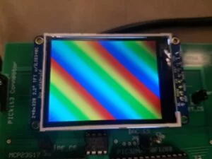
Now that the data has been processed, the data can now be output to both the TFT display and through UART. The TFT display uses the distance data as well as the ADC unit values after passing through the Kalman filter. By using the azimuth measurement as an X coordinate and the altitude measurement as the Y coordinate, a pixel at the specified coordinate is written. The color of this pixel is determined by the distance value. As discussed below, an array of 188 values was calculated with 0 being a value to display blue on the TFT, 188 being a value to display red, and the values in between being a rainbow pattern from blue to red. By multiplying the distance measurement by 188 and then dividing by 600, the distance data is mapped into the array so that a very close value is blue and a value as far away as 6 meters is shown as red. By writing these points to the TFT, a real-time distance map is created. This real-time feedback was extremely useful when trying to tune the system.

To send data over UART, a specified buffer, PT_send_buffer, was written to using sprintf. Then, a thread was spawned to set up a DMA transfer of this buffer to UART. This created a non-blocking way of writing to UART. On initialization of the analysis thread, the header for a PCD file, a point cloud data file format, is sent line by line over UART. Once the thread starts processing data, the cartesian points are sent through UART. The cartesian points are writen in the format “X, space, Y, space, Z, end line” in compliance with PCD formatting. The result was that all of the lines a computer received from the PIC32 could then be saved as a PCD file and displayed as a data cloud set, resulting in a 3d image.

As an aside, the color array used for the TFT display was initialized at start up of the system. The TFT color format is 16 bits with the top 5 bits the red intensity, the middle 6 bits the green intensity, and the bottom 5 bits the blue intensity. In order to create the rainbow array, I started with a value which correlated to pure blue. I incremented the green intensity to full, followed by decrementing the blue intensity to zero, followed by incrementing the red intensity to full, followed by decrementing the green intensity to 0. At every increment or decrement, the value was stored in the color array. The result was an array with a rainbow of color from index 0 to index 188. As an example of using this array, the below TFT display was made by simply running through the color array.

Hardware Overview

The hardware consisted of the circuit to provide power to the two servos and the lidar, the circuit to trigger the lidar sensor, the differential amplifying circuit for the analog feedback from the servos, and the mechanical hardware to mount the lidar circuit and the two servos. In addition, a UART serial to USB cable was used which both provided 5V power to the circuit as well as allowed for UART communication.

Mechanical Hardware

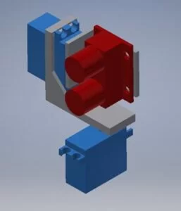
The mechanical hardware consisted of two mounting brackets to mount the altitude servo on the azimuth servo and then to mount the lidar sensor onto the altitude sensor. The CAD design for this is shown below. The main goal behind this mechanical design was to allow for unobstructed rotation for the lidar sensor as it moved through the scan pattern. The lidar needed to be rotated without ever having the mounting in the way of the laser. Additionally, this mounting system needed to make sure that the lidar was mounted at the center of rotation for both the azimuth servo and the altitude servo. If the lidar sensor is not mounted at the center of both axes, then the distance measurement will not truly be the radius in spherical coordinates. This would cause multiple other complicating factors and would have to be fixed by very complex and computationally intensive math. To avoid this, the mechanical design has built in micro adjustments for both the altitude servo mounting and the lidar mounting. Both components are mounted by using screws and nuts, but the hole for these screws is an open slot. This allows the screws to be positioned in a range of positions before fastening the washers. This is all to ensure that the lidar is at the center of rotation. Finally, the azimuth servo was attached to a wooden mount which was simply 2 blocks of wood screwed together. This kept the structure stable due to the mount’s weight, and duct tape could be used to mount the wooden stand to the table or floor if any shaking was seen.

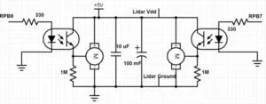
Power Circuit

The purpose of the power circuit is to provide power to both the servos and the lidar while trying to reduce any harmful noise coming from the servos. The servos produce electrical noise which can possibly damage the lidar sensor and the MCU, so precautions had to be taken to mitigate this effect. The diagram for the power circuit can be seen in Figure 1 of Appendix B. This circuit uses two optoisolators between the PWM output from the PIC32 to the control signal input of the two servos. Also, this circuit uses two capacitors, one ceramic and one electrolytic, connected across the rails. This is an attempt to mitigate electrical noise by having the ceramic capacitor filtering out the smaller, quick noise and the electrolytic capacitor filtering out the larger, slower noise spikes. The power is connected to the 5V pin coming from the UART cable, and the devices all share a common ground with the PIC32 so that the analog feedback from the servos is useable.

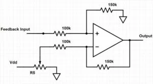
Differential Amplifier

Two differential amplifiers are used to amplify the analog feedback from the servos. The analog feedback, without amplification, only varies from around 1V to 1.7V. This would limit the resolution of the measurements of the servos’ positions, so this signal needed to be amplified. The two differential amplifier circuits can be seen in Appendix B, figures 2 and 3. The circuits are the same except for different resistor values; the circuit for the altitude servo is designed to amplify the difference by 2 whereas the circuit for the azimuth servo amplifies the difference by 1.5. This is due to the azimuth servo having a slightly larger range of voltage values caused by this servo moving slower than the altitude servo. The voltage for the negative input of the op amp was found by hooking up the differential amplifiers to the servo feedback and then displaying the output on an oscilloscope. The potentiometer was then adjusted until no clipping occurred. The result is a feedback signal which had a greater range of ADC units.

Lidar Circuit

The lidar circuit was extremely simple; it consisted of a single resistor. The lidar sensor works by hooking one wire in the configuration shown in Appendix B, figure 4. Driving the line low triggers the lidar sensor to take a distance measurement; the lidar then outputs a PWM signal onto that line as an output. The resistor is in place to avoid contention between the trigger signal and the lidar output. For this project, however, the lidar needed to constantly take distance readings. That is why one side of the lidar is connected to ground instead of an output from the PIC32. Since the line is always driven low, the lidar will constantly take distance measurements.

Results

The end result of this project was a functioning 3d imaging system. In order to create a good 3d image, the system needed to run for about 2-3min in order to capture between 10,000 and 15,000 cloud points. A video of the TFT on start up can be seen below. The distance map clearly shows a blue section in the bottom left hand corner for the table, a teal shape which correlates to the black chair slightly further away, a red section correlating to the seeing through the windows in the lab, as well as many other features.

Below is a distance map alongside a picture of what the system was pointing at. Again, multiple features are clearly visible in the distance map of the actual scene. A distinct blue shape is seen for the chain as well as the red shading around it which discerns the far wall. Also in this distance map is a clear view of a vertical pole holding up a shelf over a desk. This pole is about 1.5 inches wide and is maybe 3 meters away from the system, but three are clearly teal points marking the pole on the map. This shows the resolution to which the distance sensor can resolve objects.

Below are several 3d images created using the output of the system over UART as well as pictures of the scene being scanned. If you have a .pcd file reader, such as Matlab, you can view the 3d image by downloading the. pcd file in Appendix C. There are several features shown which are important to take note of in the 3d image. The first is the triangle bracket. This shows, again, the precision of the system when detecting narrow objects. A second feature to take note of is the trash can. The trash can is relatively close to the back wall, yet it is clearly distinct from the other objects and it has a distinct rounded face. Finally, both the flat ceiling and floors as well as the flat cabinet face are important features. When converting from the polar coordinate data into cartesian points, things can end up looking curved if the conversion is not done correctly. The noticeably flat vertical and horizontal planes show that the conversion to cartesian points is indeed working correctly.

The generated 3d image clearly correlates to the image seen by the sensor, though the budget in the design is apparent. The 3d image takes a couple minutes to be created, and the resulting image does not clearly show what the system has seen. It is possible to recognize objects in the 3d image after looking at a picture of the view, but it is more difficult to discern what is in the scene by only looking at the 3d image. Object detection however, if not object recognition, could still be possible with this design, and these results are expected for a project with such limited resources.

Conclusion

This project went well in the end. The biggest thing that I hoped to come out of this project was a proof of concept that useable data could be taken from this very low budget lidar imaging system. As shown in the results section, the 3d images do produce meaningful data. Objects can be detected using the system, and the distances to these objects are measurable. Should this project be put into a data collection system, this sensor could be used in tandem with another sensor, say a video camera. The images from the video would be useable for analysis such as object recognition, and this component could be used to determine distance of the object and general three-dimensional shape. This system would perform better for mainly stationary scenes with minimal motion due to the time required to create an image, but distance measurements could be taken if the FOV of the lidar scanner is matched with the FOV of the camera so that individual time stamped cloud point datum could be matched with pixels in a video frame.

If I had additional time to rework this project, the first thing that I would change would be the servos. The servos worked as expected; they were kind of slow and shaky. However, they reliably moved through the scan pattern and were easily controlled. I believe the biggest factor causing the noise in the images produced is from the jittering of the two servos. If a bigger budget was available, more advanced servos which could both move quicker and move with less jitter and unwanted motion could be found. This would not increase the budget by too much while greatly increasing the quality of the images produced. Higher quality and faster servos would also ecrease the time required to create a decent image. I believe this change would increase the usability of this system without pricing it out for too many potential data collection projects.

Intellectual Property Considerations

As for IP considerations, nothing in this project is patented or trademarked. The idea behind rotating a distance sensor through a scan pattern to create a 3d image is widely known and used, and the use of servos to perform this action is again a widely known procedure that is not copyrighted. As for code, I wrote all of the code in the lidar_system_code.c file listed in Appendix C. The header file, config.h, is a slightly modified version of code which was written by Bruce Land. The include file pt_cornell_1_2_1.h which supported things such as UART communication and threading were also provided by Bruce Land [2]. Because nothing in this project is inherently new or novel other than my specific implementation of the idea, nothing for this project is patentable. However, the steps taken to design and build the lidar scanner could possibly be publishable for a magazine or journal.

Code of Ethics

First and foremost, this project was designed with consideration of other peoples’ health and wellbeing in mind. The main source of possible problems was the use of the laser. Certain lasers can cause damage to eyes or even skin if they are powerful enough. The laser used for this project, however, was a Class 1 laser. This means that the power output by this laser is low enough that even direct eye contact with the laser, while not advised, is shown to not cause any harmful effects. The lidar sensor was kept intact without any hampering of the internal structure, so it is perfectly safe without any additional precautions. Furthermore, I have tried to be as honest as possible about both the results seen from this project and about the work behind this project. I have written almost all the code and have designed all the hardware with the exceptions listed above in the IP considerations sections. All the pictures and results shown are also unaltered pictures created by this system. No results from other peoples’ systems were shown and no doctoring of the images and results were done to try to show a better result than actually achieved. Finally, while I have worked in the past for a company developing a lidar system, I made sure that none of the proprietary designs or ideas of that company were used for this project.

Legal Considerations

There are not many legal considerations for this project. As mentioned in the Code of Ethics section, the laser being used is a Class 1 and thus does not require any specific safety measures or limiters. Other than the laser, there is nothing about this project that could be controlled by legal restrictions.

Circuit diagrams

Source: ECE 4760 Final Project: 3d lidar imaging system