Rubot

Introduction

Almost everybody has used a rubik’s cube puzzle before, whether they are picking up the cube for the first time, looking up the solution algorithms, or playing around with a different iteration. Many different kinds of rubik’s puzzles have come out over the years, such as the Rubik’s Cube Pyramid and the 2-by-2 cube Rubik’s Cube. The most common of these puzzles is the original 3-by-3 Rubik’s Cube. For our final project, we made a Rubik’s Cube solver that can guide people how to solve their Rubik’s Cube after they have been scrambled.

High Level Design

In order to operate Rubot, a user must take a solved cube first and scramble it with a set of moves. The user then sends the move set to the PIC32 using a python GUI for the cube to be solved. The PIC32 then proceeds to solve the cube and generates a solution move set. Finally, the solution moveset is displayed on a TFT screen that is attached to the PIC32. The solution moveset displays one move at a time and the user can go to the next or previous move in the moveset by using buttons on the GUI.

Hardware

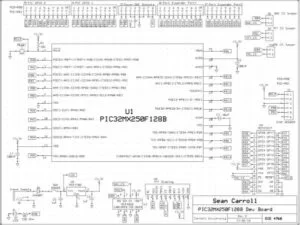
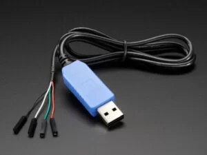
There are two hardware peripherals in our design: the TFT display and the UART to USB Adafruit serial cable (used for the GUI). To hook up the TFT display, refer to the board schematic in Appendix C. The TFT is labeled as U5 on the schematic. Next, to hook up the UART to USB serial cable, attach the following wires to the designated pins on the board:

A visual reference and a link to purchase the UART to USB serial cable in given in appendix C.

Software

The software is broken down into 3 modules: solver, gui, and pic32. The solver module implements the Rubik’s cube solving algorithm and associated state, the gui module implements the Python GUI to communicate serially with the microcontroller, and the pic32 module implements hardware-specific code including for the TFT display. Each module was designed, implemented, and tested independently.

solver Module

Cube State

The 26 minature cubes that make up a full Rubik’s cube are called cubies. Every Rubik’s cube has 12 edge cubies that can be in one of two orientations, and 8 corner cubies that can be in one of three orientations. Since the 6 face cubies are not affected by face rotations, we only encode the edge and corner cubies in our cube representation. We enocde edge cubies using 5 bits (first bit encodes orientation, next four bits encode permutation), and corner cubies also using 5 bits (first two bits encode orientation, next three bits encode permutation). Then we encode a cube state with two 64-bit integers, the first integer encoding the 12 edge cubies sequentially, the second integer encoding the 8 corner cubies sequentially. To read the value of an arbitrary cubie, we simply select the appropriate integer and read the orientation and permutation at the index of that cubie.

Moves are what cause transformations between cube states. Each move must specify the face of rotation; and also specify whether the rotation is a quarter-turn clockwise, quarter-turn counter-clockwise, or a half-turn. We encode the face of rotation for a move as a one-hot encoded 6-bit integer. We encode the rotation value as a one-hot encoded 2-bit integer where the rotation is quarter-turn clockwise by default, one bit flag makes the rotation counter-clockwise, and the other bit flag makes the rotation a half-turn. Then we encode a single move as an 8-bit integer where the first 2 bits encode information about the rotation value, and the last 6 bits encode information about the face of rotation.

Finally we implemented a transformation function which takes a cube state and a move, and returns the new cube state obtained by applying the move to the original cube state. Decoding moves is relatively simple given their encoding. Each move requires shifting the permutations of four edges and four corners, which is also relatively simple. Updating the orientations of the edges and corners was the tricky part that required a lot of trial and error. As it turns out, edges flip their orientation on rotations of two arbitrary opposite faces, which we selected to be the U and D faces. Corners change their orientations on rotations of four arbitrary opposite faces, including the U and D faces. We selected the other pair of opposite faces to be the F and B faces. The value by which their orientations change depends on the which corner they started in on the face of rotation.

Building the cube state model required a lot of testing between incremental improvements. Much of our testing came from taking a solved cube state, applying a random sequence of moves, and printing it to the console. Then we applied the same sequence of moves to a real Rubik’s cube and verified that the faces all looked the same. We performed this test hundreds of times on randomly generated sequences of moves before we were convinced our model was working correctly. We also added some automated tests which verified that communicative moves produced equivalent states, and that certain move sequences when applied to a solved cube would produce a solved cube after a pre-computed number of steps.

We went through many different iterations of potential cube state models. We initially chose to represent cubes as a 54-element array, which maps a square on the cube to its current color. This turned out to make the actual cube solver much harder to implement, since the algorithm relies on cubie orientations and permutations. Therefore we found the above model to be most natural for implementation of the cube solver algorithm.

Cube Solver

The Rubik’s cube solving algorithm we chose to implement is an improved version of Thistletwaite’s algorithm. Thistletwaite’s original algorithm is guaranteed to find a solution within 52 moves, while our improved one can find a solution within 46 moves. Thistletwaite’s algorithm is an improvement over brute-force search algorithms which would never terminate in such an overwhelmingly large state space, and over ineffecient human algorithms that freqently break properties that are built up in previous stages while progressing towards the next stage. It is a relatively complicated algorithm that is only practical for computer solving and not for humans to memorize.

Thistletwaite’s algorithm is better explained by rudimentary group theory. It divides the space of cube states into 4 nested groups, where a group is defined by a set of moves and contains the set of cube states that can be solved using that set of moves. The algorithm progresses in 4 phases, where phase i aims to bring a cube from group G(i-1) to group Gi only using the set of moves in group G(i-1). Restricting the set of moves that can be applied to the cubes in a group fixes properties of the cubes that cannot be broken once that group is reached. The four groups of Thistletwaite’s algorithm and the fixed properties of their cubes is given below:

Group	Max Depth	Number of States	Fixed Properties
G0 = {F, B, L, R, U, D}	7	2048	None.
G1 = {F, B, L, R, U2, D2}	10	1082565	Edge orientations.
G2 = {F, B, L2, R2, U2, D2}	14	352800	Corner orientations, edges in middle slice in correct slice.
G3 = {F2, B2, L2, R2, U2, D2}	15	663552	Edges in correct slices, corners in correct tetrad pairs.
G4 = I = {}	0	1	Solved cube.

Each phase is implemented as an iterative-deepening depth-first search (IDDFS) over the state space of cubes in the current group. We implemented a single search function that runs IDDFS once for each phase, and three helper functions that provide phase-specific details to the single search function. Two of these helper functions return the moves and maximum depth allowed in a phase. The third helper function takes a cube state and returns a modified cube state where everything that isn’t related to the properties being fixed is removed. Essentially it reduces a cube state to its phase-equivalence class, so two different cube states are considered equal if their phase-specific properties are equal. These helper functions allow the phase-specific details to be factored out of the function that handles IDDFS.

The most constraining feature of the microcontroller in implementing our algorithm was the small memory size. We initially intended to implement the search as a bi-directional BFS because it would have had to search over much fewer states. But after some basic computations we realized the microcontroller simply did not have enough memory to support such a search. Instead we turned to an IDDFS search because it simulates BFS, ensuring each returned solution has minimal length, and because it runs in linear space. Since the largest branching factor of a search is 18 in phase 1, and the largest possible depth of a search is 15 in phase 4, we only needed to allocate a size of 18*15=270 to the search stack. Each search node uses 24 bytes to store a cube state, parent move, and depth. This means the memory requirements of our IDDFS search is under 6.5 kB.

In order to test the cube solver, we wrote a test function to randomly generate a cube, find a sequence of solution moves using the solver, and apply the sequence of solution moves before verifying that the resulting cube is solved. We ran this function on hundreds of randomly generated cubes before we were conviced that the solver generally worked. We also made sure to test the solution sequences on a real Rubik’s cube.

gui Module

Python Serial GUI

The user interface was designed with ease of use in mind for the user. With only four buttons and one input field, this goal was achieved. To use the GUI, a user types in a defined set of moves that would be explained in a user manual. These moves are: F, R, U, B, L, D, F’, R’, U’, B’, L’, D’, F2, R2, U2, B2, L2, D2. This nomenclature is very common among the rubik’s cube community. A user scrambles their cube and writes down each move they’ve chosen to make and inputs this move into the “Move Input” input field. The user clicks solve and then the solving moves are flashed to the TFT screen of the PIC32. A user can then step forwards and backwards through the solving moves using the “TFT Controls” buttons.

The Python interface also must parse the user input in the background before sending it to the PIC for processing. When the user clicks “Solve”, the GUI takes the user’s input and turns each move into an element in an array. Then, each move in the array is converted into an 8-bit binary representation. Finally, the array is encoded and a header, the number of moves, and a terminating character is added. This encoded “package” is then sent to the PIC32 via the UART serial connection.

The next, “>”, and previous, “<”, move buttons work in the same way as the “Solve” button except only the header and terminating characters are needed because button differentiation is done with the header characters.

pic32 Module

TFT Display

As they are going through the solution steps, the user is shown what number step they are on, as well as the next move they should do. In addition to this, we also wanted to give them a reference for what their cube should look like after each move. The graphic is made up of two images, each showing three sides of the cube. The locations of the faces on the images are based on how the cube appears when it is looked at from the orientation of the images.

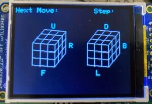
The representation of each face includes two opposite edges and nine unsigned short color values named color0 through color8. These values determine what color a given square on a face is drawn. The color of the square in the 0 position is color0 and the color of the square in the 8 position is color8. The following image shows how the positions of squares on a face are determined.

In order to color a face, the coordinates of the face and the square position are used to determine where the color should go. Parallel lines of the given color are drawn across the square to give the appearance of a full square of color.

Results

While the cube solver worked correctly, it’s main issue is that it is painfully slow on sufficiently complex cube states due to using IDDFS to search the massive state space in essentially a brute-force fasion. The number of nodes IDDFS needs to search increases exponentially with depth. More specifically, the number of nodes n IDDFS needs to search at a depth of d is given by: n=b^d, where b is the branching factor of the tree (i.e. number of moves allowed in the phase). So if the minimum solution size of a phase is sufficiently long then IDDFS needs to search a huge number of nodes to discover the solution. There are a number of improvements we can make to the system in the future to make it run faster.

The first improvement is keeping a hash table of visited cube states and pruning them from the search tree if they are encountered again. This would have the result of effectively reducing the branching factor of the search tree. For example, in G0 the branching factor would reduce from a hard 18 to about 13, allowing deeper levels of the tree to be accessed more quickly.

A more general improvement would be to generate a lookup table for each state of each phase. The lookup table would be indexed by the phase-equivalent cube state and would store the depth of a solution from that cube state. Then the solving algorithm would simply walk through the lookup table and select the next move as any move which decreases the solution depth. Such an algorithm would run in constant time, but also require generating a lookup table before use. Generating such a lookup table would take a substantial amount of time and require a substantial amount of space.

The folowing video shows the cube image graphics updating.

Conclusions

Reflection

Originally, we wanted to make a fully functional Rubik’s Cube solving machine where an unsolved cube could be placed into it, and the machine would solve the cube without any additional human interaction. We knew this would be a lot to get done though, so we first set our sights on making a Rubik’s Cube solving guide. We are pretty happy with how our project turned out, but if we were to do it again, we would want to make sure to have the graphics fully integrated with the rest of the project. We might also focus more on providing the user with a way to designate the cube’s initial state, so that they do not need to always start with a solved cube.

Considerations

Because our project is essentially a puzzle solver, we do not think there are that many facets of it that require taking ethical, legal, or safety considerations into account and we believe it adheres to the IEEE Code of Ethics. The one ethical consideration that could be taken into account when using our project, is that it might take away the enjoyment someone might experience learning to solve the cube on their own. Another thing to note though is that someone could become upset using our project if they make a mistake and do not follow the solution steps exactly and their cube is not solved at the end of the move sequence. At that point they would either have to undue all the moves they had done up to that point, or solve their cube without the guide and then start over.

Appendices

Appendix A: Inclusions

This group approves of this report for inclusion on the course website.

This group approves the video for inclusion on the course youtube channel.

Appendix B: Code Listing

Commented code can be found at this GitHub repo.

Rubot

Appendix C: Schematics

Board Schematic:

UART to USB Adafruit serial cable:

Source: Rubot