
This project aims to implement an electronic tuner which is able to analyze sound samples and display the notes contained in the sound. It utilizes a PIC32 microcontroller, a microphone circuit, and a TFT LCD to achieve that purpose.
The intuition of making this project came from the musical experiences of both of us. We are both musical instrument players in the real life, and we have to deal with tuners all the time to make sure our instruments could play the correct notes. Thus, we decided to give current commercial tuner devices a challenge and build a tuner of our own.
High Level Design
Our electronic tuner uses a microphone circuit to pick up input sound signals. After being amplified by an op-amp, the signal goes into the PIC32 microcontroller’s analog-to-digital converter (ADC) unit. Then, for each target frequency, PIC32 runs Goertzel algorithm on the recorded samples to obtain the frequency response. Since we want to know the note contained in the sound, the target frequency would have to scan through all the frequencies of notes. It would be extremely computationally expensive if we scan the entire human hearing frequency range with some precision (say 20 Hz). The reason behind is that for each target frequency, the Goertzel algorithm has to do many calculations based on hundreds of input sound samples. As the program scans through all note frequencies, the note with the largest amplitude is preserved. The note is then displayed on the TFT LCD.
Additionally, we also want to know how much off the input sound sample is from the closest note N. Consequently, the tuner also needs to scan frequencies between N-1 and N+1 (suppose N = A, N-1 = Ab/G# and N+1 = Bb/A#). In our design, 10 steps between N-1 and N+1 would be scanned, which means one frequency every 20 musical cents would be the target frequency. The information which tells us how much the input is off would also be displayed.
Other than tuning using pitch detection, to further help us tuning an instrument, we have also implemented a function which allows us to play a sample note on a speaker. The note to be played would be typed on a PC keyboard and transferred to PIC32 via UART, and PIC32 would send out corresponding synthesized sound signal to a digital-to-analog converter (DAC) unit. The DAC output would be connected to a speaker, and the note would be played.
Other than tuning using pitch detection and frequency analysis, our tuner also provides an old fashioned mode, which simply allows the user to specify a note, and then plays that note through a speaker, so that the user could use it as a reference to tune the instrument manually based on his/her own hearing. This process involves the following steps: the user tying in the name of a note on a PuTTY terminal, the message being transmitted to the PIC microcontroller through serial UART connection, the microcontroller using DDS (Direct Digital Synthesis) to produce the sound corresponding to that note, and the sound being outputted to a speaker through a Digital-to-Analog Converter (DAC) unit.
Hardware Design
Overview
The hardware design of this lab includes four major sub-circuits: the serial UART connection between the microcontroller and the PC, the microphone circuit that is used to take sound signals for frequency analysis, the audio generation circuit to output the DDS sine wave corresponding to an user-inputted note, and the TFT LCD screen to display the user interface and the results of tuning.
Microphone Circuit
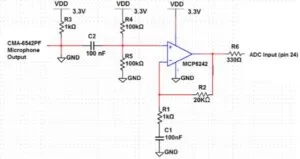
To collect sound data for frequency analysis, the microphone circuit is built as shown in Figure 2 below. The microphone CMA-6542PF is used because it is the most readily accessible one from the ECE lab. As shown in the Figure, the microphone circuitry consists of the input from the microphone, which goes through a high pass filter by capacitor C2 and a parallel of resistors R4 and R5. The cutoff frequency of the high pass filter is given by 1/(2*pi*C2*(R4||R5)), which is calculated to be 31.83 Hz. Since the lowest note on a piano keyboard C1 has frequency of around 32.6519 Hz, all the other notes will then be in the passband of the filter, which is what we desired. The high passed signal is then fed into a MCP6242 op amp, and the gain is configured to be around 20, which is reasonably large while still avoids clipping. Then the final output is fed into the ADC input on PIC32 (pin 24), in series with a 330 Ohm resistor to offer protection to the pin, where the analog voltage signal is converted to a range of 0-1023, which is then processed by our software unit.:
Audio Generation Circuit
The audio generation circuit consists of three components: an SPI DAC (Digital to Analog Converter), an audio jack, and a speaker.
DAC
As we will discuss in later sections, the sine wave generated using the DDS strategy is a digital signal. For it to be outputted through a speaker, the digital should first be converted to analog voltage levels. This conversion is done using the MCP4822 SPI DAC, which has the DAC resolution of 12 bits. The pinout for the DAC is shown below in Figure 3.
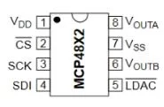
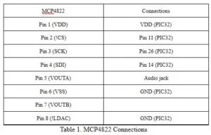
For convenience of illustration, a table mapping the connection for each pin is presented below in Table 1.
SPI channel 2 is used for the communication between the DAC and the microcontroller. On the PIC32 side, the pins for SDO2 and CS are configured and mapped accordingly using the following commands:
PPSOutput(2, RPB5, SDO2);
mPORTBSetPinsDigitalOut(BIT_4);
mPORTBSetBits(BIT_4);
SpiChnOpen(spiChn, SPI_OPEN_ON | SPI_OPEN_MODE16 | SPI_OPEN_MSTEN | SPI_OPEN_CKE_REV , spiClkDiv);
Note that MCP4822 DAC supports two output channels, while for this lab we will only use channel A, and channel B is left unconnected.
Audio Jack and Speaker
A 3.5mm audio jack is responsible to send the output analog signals from the DAC to the speaker. It is connected to channel A of the DAC (pin 5) and GND. A Logitech speaker set is provided during the lab, which is used to output the sound for the generated tone.
Serial UART Connection
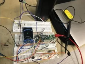
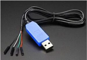
In this project, a serial UART connection is setup to send commands from a PC keyboard to the PIC32 microcontroller and direct it to perform certain functions. The serial UART communication is enabled by using the serial USB cable to connect the PC and the microcontroller. As shown in Figure 1 above, the blue serial-USB connection is a USB cable with embedded USB/serial bridge chip with 3.3 volt logic levels. The green wire is connected to the UART receive pin on the microcontroller (pin 22), the white wire is connected to the UART transmit pin (pin 21), and the black wire is connected to microcontroller ground. The other side of the USB cable is plugged in a PC USB port, and a PuTTY terminal on the PC is launched for interaction. A baud rate of 9600 is used on both side to allow proper transmission.
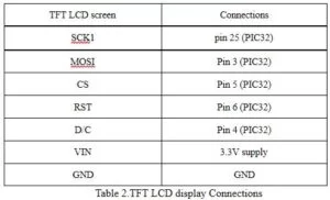
TFT LCD display
The Adafruit TFT is used for the user interface. The connection between the TFT and the microcontroller uses SPI channel 1. The mapping of connection is shown below in Table 2.
Software Design
Overview
The software design of this project relies on the protothread library provided by Professor Bruce Land and the TFT library by Adafruit rewritten by Syed Tahmid Mahbub. The design could be divided into five sub-components: the UART interaction to acquire and execute command, the ADC reading to record the sampled sound data, the frequency analysis which performs the Goertzel algorithm, the tone generation using Direct Digital Synthesis, and the TFT display.
Sampling
To get the data from the microphone circuit and convert it into the digital signal for further analysis, the built in ADC of PIC32 is used. The detailed setup of the ADC is shown below:
CloseADC10(); // ensure the ADC is off before setting the configuration
#define PARAM1 ADC_FORMAT_INTG16 | ADC_CLK_AUTO | ADC_AUTO_SAMPLING_OFF
ADC_FORMAT_INTG16 sets the output format to be integer.
ADC_CLK_AUTO sets the trigger mode to be auto.
ADC_AUTO_SAMPLING_OFF set the sampling to begin with AcquareADC10().
#define PARAM2 ADC_VREF_AVDD_AVSS | ADC_OFFSET_CAL_DISABLE | ADC_SCAN_OFF | ADC_SAMPLES_PER_INT_1 | ADC_ALT_BUF_OFF | ADC_ALT_INPUT_OFF
ADC_VREF_AVDD_AVSS sets the Vref+ to be VDD and Vref- to be VSS.
ADC_OFFSET_CAL_DISABLE disables offset test.
ADC_SCAN_OFF disables scan mode.
ADC_SAMPLES_PER_INT_1 takes one sample per interval
ADC_ALT_BUF_OFF uses single buf
ADC_ALT_INPUT_OFF turns of alternate mode
#define PARAM3 ADC_CONV_CLK_PB | ADC_SAMPLE_TIME_5 | ADC_CONV_CLK_Tcy2 //ADC_SAMPLE_TIME_15| ADC_CONV_CLK_Tcy2
ADC_CONV_CLK_PB sets to use peripheral bus clock.
ADC_SAMPLE_TIME_5 sets sample time to be 5
ADC_CONV_CLK_Tcy2 sets ADC clock divider
#define PARAM4 ENABLE_AN4_ANA
set AN4 as analog inputs
#define PARAM5 SKIP_SCAN_ALL
Does not assign channels to scan
SetChanADC10( ADC_CH0_NEG_SAMPLEA_NVREF | ADC_CH0_POS_SAMPLEA_AN4 );
configure to sample AN4
OpenADC10( PARAM1, PARAM2, PARAM3, PARAM4, PARAM5 );
configure ADC using the parameters defined above
After the ADC unit has been configured correctly, the actual sampling is achieved by setting a timer to cause an interrupt at the desired sampling frequency and read the ADC data during each interrupt service routine. Timer 2 is used for this purpose, and the its configuration is shown below:
OpenTimer2(T2_ON | T2_SOURCE_INT | T2_PS_1_1, 10000);
This command sets the timeout period to be 10000 clock cycles. Since the clock frequency is 40MHz, the resulting timer 2 interrupt frequency is 40MHz/10000 = 4 KHz, which is used as our sampling rate.
ConfigIntTimer2(T2_INT_OFF | T2_INT_PRIOR_2);
Initially, the timer 2 interrupt is turned off, and it will be turned on only when the automatic tuning mode is selected.
After the setup is done, the actual sampling is achieved in the timer 2 interrupt service routine.
void __ISR(_TIMER_2_VECTOR, ipl2) Timer2Handler(void)
In the ISR, adc_9 = ReadADC10(0) is called to read the ADC data. However, the data is recorded as (0x3FF – adc_9) (1023 minus ADC data). The reason behind is that in our implementation, ADC data is close or equal to 1023 when no significantly loud input source is present. When such an input sound source is played, the ADC data actually drops to nearly zero, and we concluded that our microphone circuit produces inverted outputs. Therefore, the minus operation is needed so that the frequency analysis may be functional.
Frequency Analysis
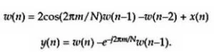
The frequency analysis is done by utilizing the Goertzel algorithm, which was recommended to us by Professor Bruce Land. It is a discrete Fourier transform algorithm (DFT) that is very fast and computationally inexpensive comparing to fast Fourier transform (FFT), while yielding reasonably reliable and accurate results.
The Goertzel algorithm is in the form of a two-step digital filter, which takes a sequence of inputs with length N:
We have chosen the sampling rate to be 4000 Hz and N to be 1000. Originally, we chose the sampling rate to be 8000 Hz, since it satisfies the Nyquist-Shannon Sampling Theorem that the sampling rate should be no less than two times the highest frequency to be detected, which is 3956.29982 Hz (B7). However, such high notes are rarely encountered by people in the real life. It also makes real-time frequency analysis more difficult to implement, since it takes only 1000/8000 = 0.125 seconds to fully record a data array. To achieve real-time frequency analysis, we would have to complete the calculation within 0.125 seconds. Nevertheless, as the late Optimization section will discuss, the 0.125 seconds constraint is actually hard to satisfy. We do not want to reduce N, since the larger N is, the more precise the analysis would be. If N is not big enough, it might result in exactly the same frequency response magnitudes for adjacent target frequencies. A large N could provide good resolution of frequencies. Therefore, we have to reduce sampling rate, and we thus have to abandon the 7th octave. A sampling rate of 4000 Hz would still be enough to perform frequency analysis on the first 6 octaves, since the frequency of note B6 is 1977.32320 Hz, which is slightly less than half of 4000 Hz.
In our implementation, the Goertzel() function is called every time we want to find the frequency magnitude of one note so that we could cover pitch detection for the entire frequency range of notes that we’re interested in. Basically, this means that the Goertzel() function is called 84 times (36 in the optimized code) for finding out which note the input sound samples resemble the most. Then, we would record the closest note and the corresponding frequency response magnitude. The sample’s proximity to a note is determined by comparing frequency response magnitudes, and the closest note should have the largest frequency response magnitude.
Moreover, since we also want to know how much the input is off from the closest note “n”, we also apply Goertzel() additional 10 times for 10 steps between n-1 and n+1. By doing this, we are basically “zooming in” to investigate the frequency range around note n. As a result, we can obtain a frequency response with better resolution around n. Then we can find out how many steps the input samples are off from n, and each step represents for 20 musical cents. In terms of frequency, 20 musical cents more than n is 2^(122/120) * n’s frequency.
UART serial interaction
For the UART serial communication part, a pt_thread is used to take in commands that the user enter in PuTTY using a PC keyboard. Input and output child threads are spawned in this thread, and PT_DMA_PutSerialBuffer and PT_GetSerialBuffer are used to send and get serial buffer.PT_DMA_PutSerialBuffer and PT_GetSerialBuffer are defined in the way that they are non-blocking, therefore whiling waiting for input or the data transfer, the input and output threads could yield to other threads.
Since the tuner needs to support two different mode, and the system needs to switch between different states to perform different functionality, a finite state machine is used in the UART thread to enable the correct handling of user inputs including the state change and the parameter setup.
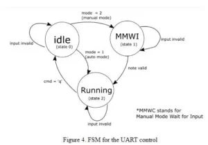
Initially, the state is set to be idle, and a prompt will be printed to the PuTTY terminal asking the user to select the mode, where mode “1” indicates auto mode and mode “2” indicate manual mode. If mode = 1, then the system will enable timer 2 for ADC reading, and the TFT display will be switched to display the note tuning meter. Frequency analysis will also be performed in the calculation thread, which will be discussed later. Also, the state machine will switch to running state, which is state 2. If mode = 2 instead, then the state machine will transit to MMWI state (state 1) to prompt the user to enter a note. If a note is correctly inputted, the note will be decoded, and the corresponding tone will be played by enabling Timer 3 interrupt. At the same time, the state machine will transit into running state ( state 2). Details of decoding and tone generation will be discussed in later sections. When the system is in running state, then whenever the user type in the command “q”, the program will quit and return to the idle state.
Tone generation with DDS
In the manual mode, the generation of the sound of reference note is achieved through Direct Digital Synthesis (DDS) technique. The basic idea of DDS is that, a 32-bit variable is used to represent the phasor of a sine wave, and incrementing this variable is equivalent to incrementing the phasor; to be more specific, incrementing the variable from 0 to overflow is the same as incrementing the phasor from 0 to 2?, and one cycle of variable overflow is just one cycle of the sine wave. That is to say, to generate a sine wave of desired frequency, f, using the timer interrupt at a frequency of 16 kHz, we could simply increment the 32-bit variable during each interrupt event, and let the variable overflow after every N interrupt events, where N is calculated by f/16kHz. The increment step that makes the 32-bit variable overflow after N increments is calculated by 2^32/N. To save memory, we decide to use a 256-entry sine table, which is created by dividing a cycle of sine wave into 256 samples and scale the samples to a range from -2048 to +2048 for future use of the DAC. Since 256 = 2^8, the top 8 bits of the 32-bit variable is then used as the index for the sine table to retrieve the sine sample.
Using this technique, we could generate the various frequencies by simply setting the increment step for the 32-bit variable to different values.
User interface and display aesthetics
For a tuner, the aesthetic traits are quite important to give the user both valuable information and an entertaining visual effect. Therefore, different from the previous labs in which the raw data are simply displayed on the TFT screen, for this project we spent considerable time designing the user interface to make it look more satisfying.
A real tuning meter like design is used for the TFT display interface. The appearance is shown in Figure 5 below.
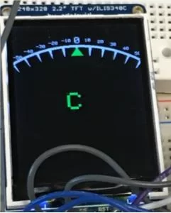
This display involves three critical components: the panel consisted of an arc and 11 equally spaced tick marks, an arrow used to point for the precision, and the actual display of the note. Careful calculations are performed, and helper functions are created to build the display.
markSetup() drawMarks() and drawCircle(short x, short y, short r, short size, short color) are the helper functions to initialize the panel. arrowIndexSetup() and drawArrow() are the two helper functions used to draw the arrow.
All these drawings include the use of the provided TFT functions for drawing circles and triangles, with the calculated index points based on the Pythagorean theorem.
Optimization
After implementing the design described above, we weren’t satisfied with the execution speed of the program. Therefore, we have come up with the following optimizations to make the system run faster:
Sampling
Record samples into two arrays (arrayID)
In our design, two arrays dataArray0 and dataArray1 are used interchangeably to store the data, and a volatile global variable arrayID is used to keep track on which array is currently used for storing. Once a data array is filled, the other array will be switched on to store new data, while the filled array will be used to perform frequency analysis. Such use of the two arrays exhibits parallelism, which essentially means that new sample could be captured while the old samples are being analyzed.
Flags
In the sampling ISR, two flags are added for indicating if each of the two data arrays is full of newly recorded samples, thus ready for frequency analysis. By adding these flags and corresponding logic in the frequency analysis code, we can make sure that by no means the DFT could be calculating upon a data array mixed with newly recorded and old samples, which is highly likely to return a wrong note. By adding data array flags to the design, we could further increase the accuracy of output notes.
Thresholding
For efficiency of calculation, we decide to set a threshold on the captured data, and any signal below that threshold will be replaced with a value of 0. We set the threshold to be 0x3FC (1020). Based on our testing, we think it is safe to conclude that ADC data larger than this threshold is caused by background noise, and thus negligible. Therefore, applying the threshold cancels noise, making the analysis more accurate.
Frequency analysis
Reduce number of notes to be scanned
Originally, we planned to cover 84 notes’ pitch detection, which means Goertzel had to be called for 94 times in total, including the 10 times for finding steps (each step is 20 musical cents) around the closest note. However, we discovered that it took too long for each frequency analysis on a data array to finish. From our measurements, it took 560-592 milliseconds to finish computing on a data array, which was not ideal since it took only 250 milliseconds to record one such array.
Eventually, we set the number of notes to detect to be 36, starting from C3 to B5. During testing, we discovered that frequencies with ~120 Hz might not be picked up correctly by the microphone, even though the high-pass filter installed should only filter out frequencies lower than 31.83 Hz. We think the high noise level might be the cause. Therefore, it would not make the device’s performance worse by removing the first two octaves. The sixth octave is removed only for increasing the computation speed, and the reason for removing the seventh octave was stated in the previous section.
After this optimization, we found the time to complete frequency analysis for one data array to be always within 200 milliseconds, mostly from 133 to ~180 milliseconds, thus making real-time frequency analysis possible.
Thresholding
We also utilized thresholding to make the displayed note less frequently to change. We set a frequency response magnitude threshold of 10^9. If the maximal magnitude of all notes’ frequencies are smaller than this threshold, the displayed note would not be changed. During testing, we concluded that only magnitudes greater than this threshold could be meaningful, and lower magnitudes are caused by noise. By applying this threshold, we could achieve that the note displayed on the TFT, the note with the largest frequency response magnitude, could be preserved on the screen even though the user has stopped to give the microphone new sound inputs.
Transforming from floating point to fixed-point
Additionally, we attempted to utilize fixed-point numbers for execution of frequency analysis. Theoretically, the microcontroller should be able to perform fixed-point calculations faster than floating-point calculations. We expected a speedup of 30-50%, since the floating-point multiplication and divisions take a significant amount of time.
In order to preserve precision, we had to use unsigned long long data types (64-bit long) to replace 32-bit floats. The reason is that the integer part of the fixed-point could take up 42 bits, since the frequency response magnitude could reach up to 3*10^12, which is just within 2^42 (4*10^12). The rest 22 bits would be used for the fraction part.
However, it did not work well for us. It seems that the microcontroller and the debugger do not function normally with 64-bit data types. A “Data Size Error!” would always appear for values of 64-bit variables. We spent a lot time debugging, but did not figure out a way to avoid this. More importantly, Professor Land told us that in reality, for our PIC32 microcontroller, 64-bit calculations might not be significantly faster than floating-point calculations, since the microcontroller is a 32-bit microcontroller. Thus, doing this floating-point to fixed-point conversion seemed pointless to us.
Testing and Results
For a live demonstration of our tuner project, please see the following video:
Project Demo
Test 1: Monotone
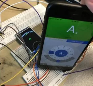
We have used a tone generator phone app to generate sounds with frequencies of musical notes to test the functionality of our tuner. The sounds are played out from the phone’s speakers. Due to high level of background noise of the microphone, the phone speaks had to be placed right next to the microphone for us to observe accurate results. It turns out that for monotone sound samples from C3 to B5, our tuner is guaranteed to display a correct note as long as the phone speakers are correctly placed, although the indicator for cents might be slightly off.
Test 2: Simulated instrument sounds
To better simulate the real-life purpose of the tuner, we have used a phone app that could generate piano sounds to test the tuner. The phone speakers still have to be placed closely to the microphone. It turns our that for most notes from C3 to B5, our tuner is able to display a correct note while the cent indicator might be slightly off. However, there are a few cases that the tuner could not display the correct note. For example, if a E4 on the simulated piano is played, a B is displayed on the TFT. We think the reason could be because of the sound characteristic of the piano or of the app that when E4 is played, the frequency with the most magnitude is a B (B3 or B4) rather than E4. This is also why it is not trivial to implement a tuner that could return correct pitches of real-life musical instruments, considering each instrument could have distinct frequency distribution characteristics.
Conclusion
Overview
Overall, the results that we obtained during testing met our expectations, considering we knew returning correct pitches of musical instruments could be hard. Of course, there are things that we can potentially further improve. The microphone circuit that we built seemed to produce too much noise, either caused by the environment or the wires and microelectronic devices near by. We could make the microphone more sensitive and accurate by reducing noise. Also, the UART transmission does not always work reliably currently, and we have not figured out the reason yet. We suspect a conflict between threads might have caused the issue.
Intellectual Property Considerations
No intellectual property would be violated in this project. All the components would be/have been purchased from legal vendors, and the software would cite any open-source or course code if used. We have used code from previous labs to setup hardware, and we also use ProtoThread to help us exploit concurrency in the project. The pitch-detection algorithm (Goertzel algorithm) is not a patent-protected algorithm.
Ethical Consideration
In regards to the IEEE code of ethics, term 1 and 9 are followed as we take the responsibility in making decisions consistent with the safety, health, and welfare of the public. The tuner in this project is safe to use since its loudness and brightness would be controlled to a level that could be tolerated by human. For term 3 and 7, we seek and accept offer honest criticism of technical work, and at the same time we acknowledged and corrected errors by admitting that the accuracy of our tuner is not perfect, and we credited properly the contributions of others by citing them in reference section of this report. This project also obeys term 8 in the IEEE code of ethics since it does not engage in any acts of discrimination based on race, religion, gender, disability, age, national origin, sexual orientation, gender identity, or gender expression. This project also shows care to the user since it would display a large font and clear indicator interface on the TFT LCD for the user to easily understand. For term 5 and 10, we try our best to help and assist others in understanding technology by writing this report, and are willing to support them in following this code of ethics. Speaking of term 4, bribery is rejected in all its forms throughout the project.
Source: Electronic Tuner Design
About The Author
Muhammad Bilal
I am a highly skilled and motivated individual with a Master's degree in Computer Science. I have extensive experience in technical writing and a deep understanding of SEO practices.